|
|
This is a slightly edited and web-friendly version of the Thesis submitted at Clarkson University in partial requirements for the author’s MS in Electrical Engineering. It is available here as a resource to those interested in learning about anaerobic digesters and their control systems. The online version omits some of the figures and appendices of the print version. A full version of the thesis is available as a PDF file here . For questions, feel free to contact Greg Linder, greg.linder@gmail.com. This document is hosted as part of many other projects by Greg, more available at at linderlabs.com's innovations section.
I would like to thank my family, my fellow Clarkson students, the Clarkson Golden Knotes, and all the faculty and staff at Clarkson University for their continued support. Specifically, thanks to Dr. Stefan Grimberg, Dr. Sue Powers, Dr. Eric Thacher, Dr. Thomas Ortmeyer, and Jill and Donna in the ECE office.
Funding for this research was provided by the NY Agricultural and Market (grant C010669), DOE (grant number DE-FG36-06G086007), USDA CSREES (grant number 68-3A75-6-512) and NYSERDA (#7848). Publication of these results does not imply endorsement of the findings by either of these agencies.
The earliest documented scientific study of biogas was presented in 1648, when Jan Baptist van Helmont described “spirits. . .coagulated after the manner of a body, and is stirred up by an attained ferment” [1]. Throughout developing countries, small scale home-use digesters are widely used for producing gas for cooking. China, for example, has 7,000,000 small scale digesters serving 4% of the population [2]. This equipment is very simple, consisting of nothing more than a covered pit and a length of pipe, with a bucket of water to act as a pressure regulator.
Systems of this sort are not directly applicable to the diverse needs of the United State’s agricultural industry. A small farm digester in India may be capable of dealing with the waste of just a few cows. These digesters often have very long residence times and require frequent cleaning. In order to scale up operations to the United State’s Confined Animal Feeding Operations (CAFO), where thousands of animals may be generating concentrated waste streams, more technically advanced systems are required. The United States Environmental Protection Agency (EPA) specifies CAFOs in terms of size. For dairy operations, a “Small CAFO” is less than 200, a “Medium CAFO” is between 200 and 699, and for a “Large CAFO” means 700 or more mature dairy cattle [3].
According to the AgSTAR program, sponsored by the Environmental Protection Agency (EPA), the United States has over 700 MW worth of electrical generating capacity available from anaerobic digesters distributed around the country whose fuel supply constitutes only hog and dairy cow manures in operations classified as medium to large CAFOs [4]. To illustrate the potential monetary value of this resource, consider the 750 MW expansion project of a large coal fired power station near Pueblo, Colorado. The Comanche 3 plant, scheduled to go online in August, 2009 has an estimated initial capital cost of 1.3 billion dollars [5]. This illustrates the amount of money utilities are willing to pay for centralized base load power.
Although the digesters exploiting animal manure would be distributed throughout the United States, the monetary value of the electrical power they could produce is nonetheless significant. According to the Energy Information Administration, in 2006 the average wholesale price of electricity in the United States was $53.00 per megawatt-hour [6]. Assuming the digesters installed in the United States can reliably operate 90% of the time that amounts to over $290 million worth of electricity per year at wholesale prices. Local farm use is even more valuable. As of 2006, the average retail price of electricity in the United States was around $89 per megawatt-hour, for a savings to farmers of $490 million per year over buying electricity at retail rates [7]. According to data presented in Chapter 6, a digester-equipped 500 cow dairy operation in New York State could save a farmer nearly $73,000 per year in utility costs. Such savings could be of great value to agribusiness in the United States, if digesters could be made both inexpensive enough and sufficiently reliable to meet the demanding needs of farmers.
The key barriers to wide-scale adoption of this resource are concerns about the capital costs and associated maintenance issues. Evidence from digesters installed in the United States shows that these concerns are valid, as demonstrated by the fact that traditionally 50% of US digesters failed soon after completion [8]. Typically, if farmers were interested in running a digester the machines succeeded if their owners were able to perform regular maintenance on equipment before small problems developed into major situations. The fact is that farmers are nervous about installing this equipment. A survey of New York state dairy operations found that 87% of farmers felt that digesters being “Very expensive to install” was a concern. Additionally, approximately 30% of farmers surveyed reported “Generator engine failures”, “Pump failures”, and “Require a lot of labor time to operate” as concerns associated with digesters [9]. The experience with Sheland Farms supports the survey’s findings, as the system owner there reports at least 20 minutes a day on digester maintenance work, reaching up to several hours when equipment failures occur [10]. There are some cases of digesters even going unfixed because the installers went out of business, making it impossible for farmers to get spare parts and service [11].
However, digesters, being small-scale power plants, are capable of being remotely controlled and monitored utilizing modern control and communications protocols. These modern protocols, and the practice of using them for local load and generation control, is a burgeoning segment of “smart grid” technologies. Furthermore, once remote control and monitoring has been demonstrated and installed, the offloading of care and maintenance of the digester to an off-site service provider would be a very effective tool both in decreasing costs of operation and decreasing the perception of digesters as unreliable. Furthermore, the application of standard utility protocols to digester control would foster a growth in small companies providing digester support services, which could be a financial benefit to small rural communities.
Pursuant to the goal of deploying remote monitoring and control systems to lower digester maintenance costs and improve reliability, the author presents two years worth of projects culminating in an in-depth discussion of a low cost and highly reliable utility-standards based communications system which can be used for remote digester management. In order to provide the context for the control protocols presented, a pilot digester was employed which required the development of a reliable local digester control system. Additionally, data was gathered on failures of a commercially installed digester located in New York State, to understand the needs of a communications link on a digester, and the current shortcomings of deployed systems.
The first chapter is an overview of common waste-to-energy technologies and a discussion of the scale of anaerobic power available in the state of New York. Chapter 2 describes the Clarkson anaerobic digester pilot plants, including introductory discussions of the author-designed systems, including those for control, manure, biogas, heating, and mechanical support.
Chapter 3 offers an in depth analysis of the Clarkson anaerobic digester pilot plant’s author-designed and built control system, including presentations on both hardware and firmware. Chapter 4 presents the electrical loads of the pilot plant, organized by system and time, and clearly illustrating the shortcomings of time-based polling for load assessment. Chapter 5 presents failures associated with the pilot scale plant, their causes and data acquisition requirements to remotely diagnose the failures. Chapter 6 discusses generator outages of a full scale digester, included illustrations of how lack of a real-time telemetry link caused increased downtime.
Having established a baseline of standard failure modes and the basic channels requiring monitoring to detect and address these failures, Chapter 7 discusses the basics of smart grid technologies, and how they may be employed to gather the data required to diagnose the situations established in the first five chapters. Chapter 8 presents a brief discussion of the per failure bandwidth requirements of the anaerobic digester. Chapter 9 offers a discussion of the types of failures addressed easily via the remote SCADA link vs. those which are only addressable by local operators. Finally, the last chapter contains a conclusion. As an added feature, Chapter 11 includes an overview of design lessons learned by the author through debugging two and fully constructing one portable anaerobic digester, as well as full plumbing diagrams, electrical diagrams, and control system functional block diagrams of the Clarkson digester controller.
According the the EPA, a farm qualifies as a Confined Animal Feeding Operation (CAFO) if the animals are maintained indoors for more than 45 days out of any 12 month period and there is no sustained vegetation in the confinement area [12]. For the size of farm appropriate for digester use, this concentration of animals requires that systems be in place to manage the waste stream as a point source of pollution [13]. In the case of New York State, all dairy farms with over 200 cows are treated as CAFO farms, requiring a comprehensive manure management plan compliant with the Natural Resource Conservation Service (NRCS) NY313 Standard [14]. As a general rule, for every gallon of milk produced, three gallons of manure are produced by a dairy farm [15].
As an example of the volume of waste generated by a multi-hundred cow dairy operation, consider one Haubenschild Farms, a large Midwestern dairy. Their cattle produce around 27 gallons of manure slurry per day per cow, with a range between 15 and 30 gallons per day depending primarily on whether or not the cows are lactating [16]. Using approximately 500 milking cows for a baseline anaerobic digester and assuming 30 gallons per day amounts to around 15,000 gallons of manure slurry per day. Manure slurry includes cow manure, bedding material, and anything else that happens to be collected in the barn manure collection system. Key characteristics of common dairy manure, as found in sand-bedded dairies in northern New York State, is presented in Table. 1.1 [17].
|
Dealing with this amount and type of material poses a challenge for any dairy operation. Additionally, manure poses a great deal of smell and mess which may can cause aroma issues for surrounding neighborhoods. What follows is an overview of four currently valid technologies for dealing with farm waste streams. All of these technologies require some sort of front-end manure handling systems. The complexity of these systems could be as simple as a mechanized front end loader to scope up manure into a pile, or as advanced as systems to separate sand and solids for various further pre-processing. The following sections are meant to be a general overview of current manure handling practice.
The most common method to dispose of dairy manure is spreading the material on arable land in order to return nutrients to the soil [18]. This is done as part of a larger Comprehensive Nutrient Management Plan (CNMP), which includes considerations for water runoff, commercial fertilizer application, and other soil and environmental issues [19]. In order to implement these plans, farmers will often store manure in lagoons for varying periods of time. These lagoons may provide up to six months of storage or down to just a few days, depending on the herd size and the CNMP [20].
While the CNMP can deal with excess nutrients and groundwater runoff, there are other issues associated with spreading raw manure. Perhaps the most obvious to those who live in dairy country is the odor from dairy operations which can be exacerbated by spreading [?]. However, in addition the the obvious odor, raw manure spreading also introduces numerous pathogens into the environment including protozoans, bacteria, and enteric viruses [22]. An effective animal manure handling system must therefore deal with both nutrient release to the land and human health issues. No matter what sorts of steps are taken to deal with environmental and pathogenic issues relating to manure, the volume of material still ends up being returned to either the land or air in some manner.
In the following sections, the processes are ranked in order of moisture content, from lowest moisture content at time of use (direct combustion), to highest (anaerobic digester).
Direct combustion of animal manure has been used since antiquity as a building material and cooking and heating fuel [23]. Even today, one former member of the Clarkson Biomass group has immediate friends and family in Africa who commonly use animal manure for heat and as a construction material [24]. In this application, the cow manure is simply left in the field until sufficiently sun baked, and then brought in and lit on fire, where it burns slowly with an even flame.
In the United States using manure for construction and cooking fuel is not necessarily a valid option. However, despite this, there is at least one vendor who offers a farm-scale direct combustion system for getting rid of manure. With the Skill Associates Elimanure system, the solid component of the manure is separated, dried, and burned in a boiler to generate steam to run a turbine [25]. The steam from the generating plant is used as a heat source to dry the incoming manure prior to burning [26]. An example of this system was installed at a farm producing 2,200 dry pounds of manure per hour from 4,000 animal units, which when burned provides enough steam to run a 600 kW generator [27].
For sufficiently dry manure such as those produced by chicken and turkeys whose moisture content is between 15 and 30% both direct combustion and gasification are potential ways to dispose of the material. Both gasification and combustion effectively reduce the input material to ash, which is a waste product that can be disposed in a landfill or used as a building material, which could be of use to a farm with insufficient spreading area to implement a proper CNMP [28].
Gasification produces synthesis gas comprised primarily of carbon monoxide and hydrogen through a controlled high temperature reaction with small amounts of steam or hydrogen. For a very in depth treatment of the thermodynamics and history of gasification, an excellent reference is presented in [29]. The output of gasification can be used directly as fuel for a turbine or other engine, or as a feedstock for other chemical synthesis operations, such as making methanol or going through the Fischer-Tropsch process to make liquid hydrocarbon fuel [30]. There are several advantages to using gasification to make syngas instead of direct combustion to make steam, including reduced dioxin and sulfur emissions and safer and less volatile bottom ash when compared to direct combustion [31].
There is at least one commercial concern offering a gasification based system that claims to work with dairy manure, Alternative Energy Solutions (AES) [32]. It is unknown at time of writing if any of these systems have been installed or are currently operable.
As animal manure continues to get more wet, it becomes possible to use composting. Composting works best with material with a moisture content of 50% [33]. An excellent definition of composting comes from [34]:
Composting is the biological decomposition and stabilization of organic substrates, under conditions that allow development of thermophilic temperatures as a result of biologically produced heat, to produce a final product that is stable, free of pathogens and plant seeds, and can be beneficially applied to land.
Composting requires that the material be provided with plenty of air, which often times will require the material to by physically mixed, as when stacked in long rows called windrows, or continuously rotated in a drum. The natural heat generation in compost is sufficient to maintain a healthy composting system at between 45-75 degrees Celsius, with warmer temperatures being better for pathogen reduction [35].
Of note in that definition is that the focus of composting is not on producing energy or nutrient management, but on making a stable, pathogen free material for application to land. A healthy composter output looks and smells like good quality garden fertilizer.
Some farms use composting as a way to process solid waste into bedding material for re-use in the barn, possibly in conjunction with a digester [36]. This is the approach taken at Sheland Farms, discussed in chapter 6. Composting, just like direct combustion, uses mostly the solids. The liquid waste stream needs to be treated as well.
There are several vendors of large-scale composting machines, which are essentially a large rotating drum mixer through which air is drawn by a fan. These are often referred to as “In-Vessel Composters”, as they are entirely contained within an enclosure of some type. Manufacturers of these styles of composters include BW Organics, of Silver Springs Texas, L&M Compost Systems, Inc of Holland, Michigan and Green Mountain Technologies of Whitington, Vermont. These machines, like the one used at Sheland Farms, are designed to rapidly and continuously compost materials. Their operation requires far less work than manually turned windrows, but their feedstock needs to be very homogeneous to work effectively. The only energy required for a composting machine comes from the motors required to rotate the drum and feed material. The heat produced by the composting action could possibly be recovered for space heating, although the temperature is not sufficiently high for power generation.
As moisture content increases beyond 70%, the material becomes too wet for use in a composter, and anaerobic digesters become the best practical energy recovery method [37]. Contrary to composting, anaerobic digestion takes place in an oxygen-free environment. A sealed vessel is seeded with material that has a healthy quantity of bacteria, such as wastewater plant treatment effluent, and then manure is slowly added. As long as the volume within the digester stays largely oxygen-free, bacteria convert the organic carbon within the waste into methane, carbon dioxide, and some additional trace gasses. Both liquid and solid waste streams are treatable with anaerobic digestion. The output of a healthy anaerobic digester, known as effluent, has a very low odor intensity and the composition of a highly aqueous homogeneous soil suspension.
Anaerobic environments produce significant amounts of biogas, which contains predominantly methane and carbon dioxide as well as small amounts of hydrogen sulfide and ammonia [38]. Additionally, due to the wet environment of an aerobic digester, the biogas can contain water vapor and trace amounts of other gasses. The hydrogen sulfide can combine with the water vapor, producing sulfuric acid which which can cause corrosion and damage to equipment if not managed properly. Digesters can be very expensive and labor intensive to install initially, but require much less space than windrow-style composting. The technology of anaerobic digesters is comparatively simple compared to direct combustion, due to there being no steam plant associated with digesters. Also, digesters are able to work with a variety of feedstuffs, and work well with very wet materials, as is the case with dairy operations which can utilize a lot of water for cleaning in addition to the aqueous waste streams from livestock.
Certain digester operators charge tipping fees or accept other local wastes into their digesters. The Sheland Farms digester, for example, occasionally serves as a disposal location for large quantities of milk. The Clarkson Pilot plant was at one point used for digesting glycerol. This “anything that can biodegrade” to energy approach makes digesters very appealing for rural settings, as it not only deals with the manure on a farm, but also provides a potential income source if farmers chose to charge tipping fees for others to feed their digester.
Even without tipping fees, adding higher energy feed to a digester can be very beneficial for gas production. Putting nearly any biodegradable material into a healthy digester will increase its gas production when compared with manure, even such standard items as food scraps and grass clippings. For a large table of various materials and their associated biogas potential per kilogram of digested material, see [39].
A significant benefit of anaerobic digesters is that the technology offers the potential to be a reliable, renewable base-load form of power generation. Most other renewable resources, with the exception of hydro and geothermal, are incapable of generating continuously, being dependent on weather for their power production. In the case of an anaerobic digester, however, as long as the digester is kept warm and in good repair, and the farmers continue raising their livestock there will be manure generated which forms the fuel for the digester system. This gives wide-scale adoption of energy from farm waste an advantage when compared to other environmentally beneficial clean energy projects. Additionally, Anaerobic Digestion (AD) generation capacity comes mainly as a side effect of addressing other pressing farm issues, including odor control, bedding re-use, waste material consolidation, and upgrades to waste handling systems for more efficient nutrient use [40].
The EPA believes that anaerobic digesters become economically feasible at herd sizes above 500 head of cattle or 2000 hogs , corresponding with the EPA’s medium to large CAFO regulations[41]. New York State alone contains 15 MW of available generating capacity from anaerobic digesters on dairy farms of 500 head or more using current technologies, constituting 150 total farms [42]. 15 MW of electrical generation, using the average 2007 New York retail electricity rate of 12 cents per kilowatt hour represents almost $16 million worth of electricity every year. Much of this would be in avoided cost to farmers, up to about $106,000 per year per system installed. These estimates are very generous, but even so, farmers able to install anaerobic digesters that can be kept operating for long periods of time will see financial benefits.
Considering that the 15 MW of generation capacity available in New York State consists mostly of generators in the 100 kW range, this amounts to approximately 150 farms capable of dealing with anaerobic digesters. Over the entire United States, the 700 MW worth of potential capacity identified by AgStar would could be as many as 7,000 different sites. To give a measure of comparison, as of 2007 the United States had 616 coal-burning sites providing 33% of the United State’s 986,215 MW total generating capacity [43]. Even in New York, controlling and maintaining the 150 farms currently capable of supporting the equipment is a large engineering challenge.
Farming is a job which traditionally requires very long hours. Farmers are kept busy operating their farms which often requires the maintenance and repair of large equipment whose failure can result in lost revenue for the farm. Although the equipment used on digesters is similar in operation to other modern mechanized farm implements farmers may not have the time or interest in maintaining another piece of mechanized equipment. Evidence from the past indicates the scale of the maintenance problem. During the 1970’s, during the oil embargo, there was much research into anaerobic digesters [44]. As an example of the scope of this research, a literature review of anaerobic digester technologies published in 1979 includes over 100 articles, journal publications, and patents with publication dates from 1977 to 1978 [45].
Much of the equipment installed during this period broke down or failed at least partly due to operator inexperience, lack of technical support, and maintenance issues [46]. Even as late as 1998, the failure rate for continuously mixed digesters approached 70%. Overall, of all 94 digesters either built or in construction in the United States of any kind, 50% have failed since they were originally constructed [47]. Leading causes of these failures were equipment failure or poor maintenance, exacerbated by some farmers who were inattentive to their own equipment. These facts have conspired make digesters appear unreliable and expensive, which has made farmers understandably uneasy about installing them.
However, many of the failures of these early systems could have been prevented with a reliable and robust communications connection to remotely monitor and address situations before they could balloon into major system problems. When in the 1970’s the equipment was first installed, the Internet and computerized, low cost industrial control equipment were not available. With the availability of low cost industrial control hardware and nearly ubiquitous home Internet links, many of these problems can be effectively found and managed, as will be discussed in the coming chapters.
A significant problem associated with running CAFO operations is bedding material. Cows or any animals kept in confined spaces need frequent bedding changes to maintain their health. Many different materials are used for bedding, including sand, hay, shredded paper, manure solids, composted solids, and saw dust. Northern New York has a fair number of large dairy operations that use sand. It is believed by many that sand provides the best material for bedding dairy cattle. The relative merits of sand and other bedding systems are beyond the scope of this thesis, but the Cornell Waste Management Institute at Cornell University’s Department of Crop and Soil Sciences has a very complete and thorough literature review available online which summarizes the results of more than fifty papers in this area [48].
Using sand presents unique operational difficulties for running anaerobic digesters. The original impetus for the Clarkson Biomass Group was to study digester operations using sand bedded dairy cows. Sand bedding needs to be either efficiently removed from a digester or removed from the manure stream before going into the digester to prevent the digester from silting up with indigestible solids over time. In order to do this a pilot scale plant was needed which could be easily installed and re-configured for various sand separation technologies.
The evolution of the digester continues at Clarkson, and a focus has now shifted to laboratory scale experiments and verifications based on the sand-separation experiments performed using the previous pilot plants. While the focus of the research project is sand removal technologies, there is also considerable work going forward in the area anaerobic digester control and efficient design. The following sections present the systems as installed on the pilot plants so the reader can become familiar with the particular concerns of digester operation driving the coming control and power discussions.
None of the Clarkson digesters were fit with generators and their associated line-voltage AC interconnection equipment, due to their small size. There are many off-the-shelf standard control and remote telemetry solutions for generators which are available from the generator manufactures themselves. Therefore the focus is on the digester itself with the assumption being made that if reliable failure analysis can be provided to illustrate the effectiveness of remote sensing and real-time data on digester operation, then an already available generator control system can be integrated with the digester control solution.
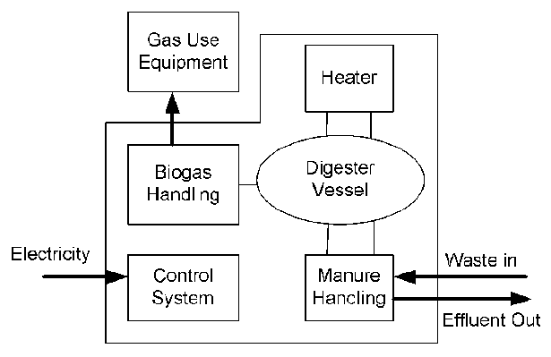
A generalized diagram of a digester is shown in Figure 2.1 which shows standard blocks common to all farm-size anaerobic digesters. All digesters require some sort of storage vessel, which needs to be sealed from the outside environment to prevent air from entering and biogas from leaving. Some vessels have built in gas storage facilities whereas others may require external gas storage in order to maintain pressure in the tank.
All digesters require some sort of heating system to maintain the temperature of the contents of the vessel near optimal for that design. Some large anaerobic lagoons may not have active heating, but still feature some form of insulation or thermal monitoring to judge digester health. More advanced systems will have multiple heat sources, possibly including in-tank or external heat exchangers supplied by engine heat or an external water heater.
Additionally, there is always some form of manure handling system. For the purposes of this research, the manure handling system is that which is used on the digester itself, including feed pumps and tank mixing systems. Whatever the farmer uses to get the manure to the point where the feed pump is responsible for it lies outside the scope of the digester.
All digesters have some kind of biogas handling system. The primary goal of this is to deal with the gas in a way optimal to the farmer’s operation. Gas handling may include any monitoring, storage, or treatment for the gas. The gas handling system is the equipment used in between the digester tank and the equipment which utilizes it. Gas use equipment could be, for example, be a prime mover for a generator, domestic home heating system, or even flaring to the environment.
A control system holds all the systems together and provides for remote monitoring and control. Ideally, a scalable digester controller will implement necessary functions to control the equipment contained in Fig 2.1. The controller developed later will allow for standard control on the basis of this block-diagram digester for a high level view of the requirements of scalable digester control.
The initial Clarkson digester was designed by Mtarri / Varani LLC of Golden, Colorado to test the operation of a means to remove settled bedding sand from within the digester tank after undergoing bio-degradation. It was thought that the sand could be made clean and removed from within a digester tank, and that raw sand-laden manure could be supplied to the digester and the solids efficiently removed. This system was operated from September 2007 through mid-December 2007 when it had to be turned off due to weather. The operation of this system was essential for design decisions which resulted in the scalable control system employed on the Version 2 digester. For readability, the diagram has been omitted from the main body, but is available in Section 11.5 [49].
The Mtarri / Varani design came with no electrical system, and a rudimentary controller and thermostat system for tank temperature control was implemented rapidly by the author before deployment, which featured limited automatic control features. Feeding and mixing were performed by operating switches on the front panel. The construction and operation of the this system, requiring frequent visits by Clarkson students to perform maintenance and take samples, clearly demonstrated the requirement for an automatic local control system. Originally, a great deal of control and monitoring hardware was purchased for this digester, but most was not installed due to considerable operational difficulties and time pressure. However, virtually all of this hardware was eventually used on the Version 2 digester.
The PLC on the Mtarri / Varani digester was used as a datalogger only, and monitored temperatures and gas properties. The measured channels included heater system temperature, tank temperatures, ambient temperature, gas flow, and methane concentration. The logged channels are summarized in Table 2.1.
|
The initial Clarkson Digester provided valuable insight into what features were required and which were not. These lessons were taken under advisement and the parts of the old digester were transformed into a new one over the winter. The initial digester was designed to test the feasibility of in-tank sand separation. It was decided that the new digester should only be for digesting, and that the sand separation would be performed outside the digester vessel itself. It was therefore decided to re-construct the Mtarri / Varani design into a new digester, whose sole purpose would be a digester and a source for reliable effluent for use in sand separation experiments. The new digester would also feature a state-of-the art control system, designed to meet the needs of the experimenters while also providing sufficient data for troubleshooting and feasibility studies related to remote operation.
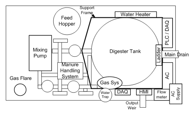
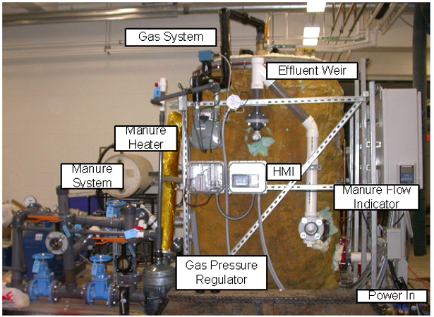
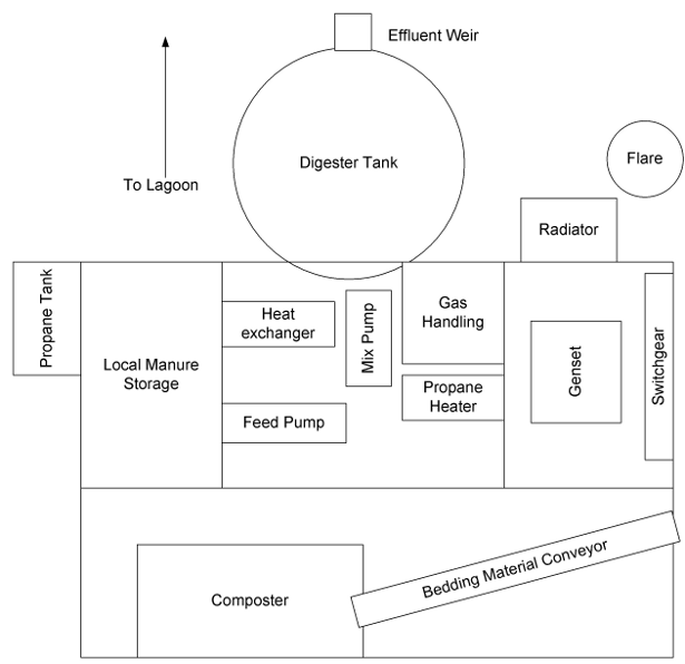
Using the lessons from the Mtarri / Varani digester, a new system was designed and constructed. Most of the new digester was a rework from the original digester, with new plumbing and manure handling systems. The control system was totally redesigned for the new digester, and all of the purchased control hardware was installed on this new version. A diagrammatic view of the new version is shown in Figure 2.2. Additionally, a side view of the digester is shown in Figure 2.3. What follows is a short discussion of each of the key systems, as follows:
This section is meant as a brief overview to familiarize the reader with the components of the digester. Much more in-depth discussion of the control system follows in subsequent chapters. In the Mtarri / Varani digester, the controller was merely used to log data channels. In the new one, the installed controller was responsible for the following operations:
As a result of the group’s experiences with the Mtarri / Varani design, it was decided that as much should be automated as possible to prevent frequent site visits. The system still needed to be fed by hand, due to the requirements of the sand separation experiments, but the system was implemented in such a way as to make this as repeatable and as easy as possible for the operators. The features included in this include a gravity-fed graduated feed hopper, automatic pump operation during feeding, and programmed regular mixing intervals without operator involvement.
Eventually, the controller was to operate in fully-automatic mode, performing its own feeding and system maintenance tasks, but this once again was delayed due to the need to get the digester back in the field for summer testing. Table 2.2 shows the telemetry channels logged for version 2. There was also an ultrasonic flow meter installed on the tank return line, which was not logged automatically by the control system due to the intermittancy of the pump operation and the very long response time of the flow meter. These values were recorded manually when the tank was fed by the operators of the system.
|
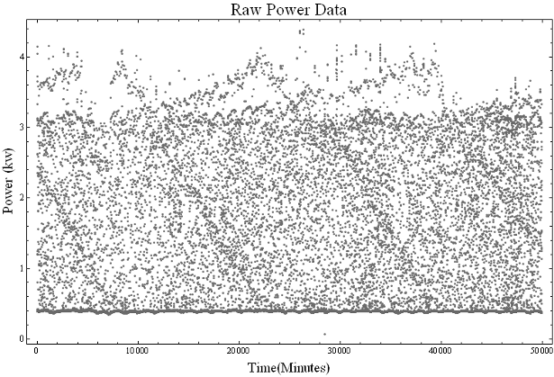
This control system worked well, giving carefree operation over the course of the whole summer. One month before the conclusion of the summer’s work, a power logger was added external to the digester itself. This was originally designed to be installed as part of the control system, but due to time constraints was not initially integrated. Post-processing of the power data from this logger is explained further in Chapter 4.
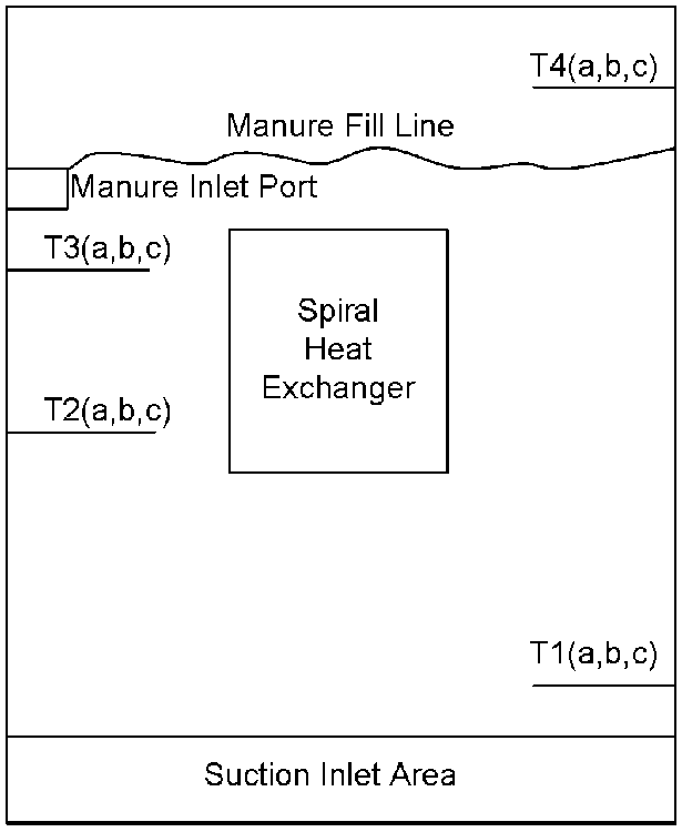
For the Initially there was significant interest in monitoring tank temperature, so the digester tank was instrumented with 12 thermocouples at varying heights and distances into the tank volume. The data from these thermocouples was to be used for comparison to a fluid dynamic model. This model has not yet been completed, and although the data was briefly analyzed by the author, it is not immediately relevant to this thesis.
Due to several thermocouples being damaged and lid access issues relating to plumbing and wiring, the new digester featured a different thermocouple layout, using fewer thermocouples in different positions than in the Mtarri / Varani design. The thermocouple positions within the tank of the version 2 digester are shown schematically in Fig. 2.4. The “abc” in the figure refers to inner to outer (a = innermost thermocouple, c= outermost). In addition to these 12 thermocouple channels, there were 4 thermocouples in the water heater system, 2 in the manure heater system, one in the manure pump, one in the gas tee, and an ambient temperature sensor, for a total of 21 temperature channels.
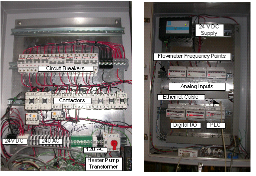
The control system was implemented primarily from parts from SixNET, a manufacturer of open-source PLC (Programmable Logic Controller) equipment and peripherals. In addition to this, standard off-the-shelf circuit breakers and contactors were installed according to National Electric Code (NEC) sizing specifications in the “AC Enclosure”, which enclosed all the line-level AC equipment. The types and quantities of non-AC related devices used in the combined controller/DAQ are shown in Table 2.3. The enclosures were all National Electrical Manufacturers Association (NEMA) 4X rated weatherproof enclosures, and all conduit and cabling was installing according to standard practice for outdoor electrical equipment.
|
The SixNET hardware was chosen primarily because of its low cost and out-of-the-box data logger functionality. Other PLC vendors were examined, but the SixNET hardware seemed to have the most features for the least amount of money. In addition, they are based in Clifton Park, New York and have very friendly and helpful staff.
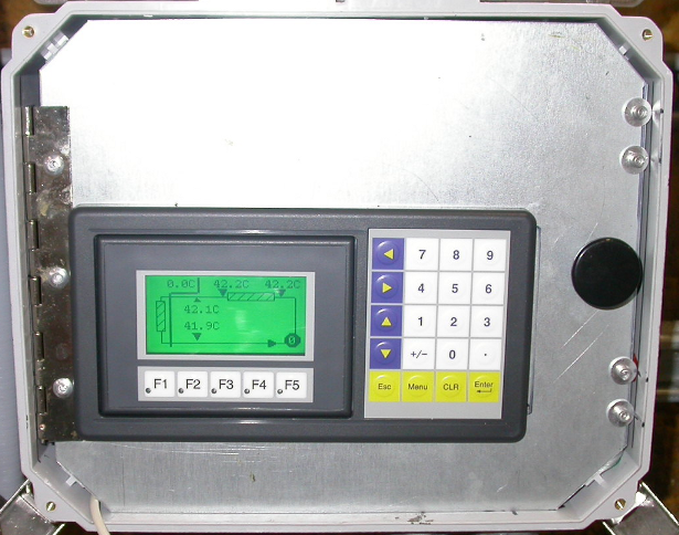
Physically, the controller occupies four weatherproof enclosures, two on the back of the unit and two on the side. These enclosures are labeled “DAQ”, “HMI”, “AC”, and “PLC/DAQ” in Fig. 2.2. The internals of the two main enclosures are shown in Fig. 2.5. At left is the AC enclosure, with circuit breakers along the top row and contactors along the center. At right is the main PLC enclosure. There are two modules mounted remotely in the DAQ enclosure to save thermocouple wiring. The HMI is mounted on the side of the tank to be at appropriate eye level for system operators.
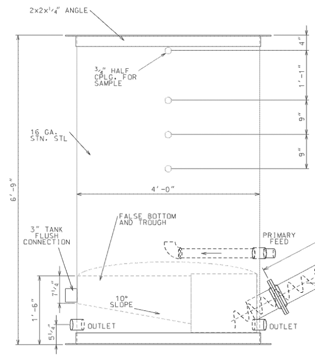
The digester tank is an integral part of any digester system. The initial version of the Mtarri / Varani is shown in Fig. 2.6[50]. Notice the false bottom and trough features. These systems were removed when the tank was refit for the version 2 Clarkson digester.
|
|
The digester tank has a height of 6’9” and a diameter of 4 feet, making its total volume approximately 634 gallons. Elsewhere, the tank is referred to as having a volume of 515 gallons. The difference is because of the need for head space in the digester tank, and the need to account of the plumbing system totals in the manure tank volume. The plumbing uses around 45 gallons to fill the pumps and 3 inch manure system.
A small volume of the digester is lost because of the internal heat exchange and related tubing in the Clarkson digester, but this amounts to less than three gallons, which is the total volume of the fluid in the heating system. Therefore the “hydraulic volume” of the Clarkson pilot digesters is 515 gallons. The head space of the digester therefore represents a volume of 164 gallons, or 22 cubic feet. Under normal operating conditions, the liquid level in the tank is then 1.75 feet down from the top.
In Fig. 2.6, this corresponds to the level of just beneath the second 3/4 inch sampling port. The actual tank delivered had an additional penetration not shown in this figure, directly opposite the line of sampling ports which was used for the effluent weir.
The feeding, mixing, and effluent output are all collectively known as the manure handling system. This includes the 3 inch diameter plumbing, large pump, valves, and other equipment used to mix the tank. For clarity, the diagram of this system has been omitted from the main body of the text. The manure plumbing system as deployed on the pilot plant is illustrated in Section 11.2.
Before describing the manure handling system, a brief discussion of the properties of sand laden dairy manure is worth presenting. For those who have not experienced sand laden manure, its consistency is similar to that of watery oatmeal, if one were to add a good cup of sand and a handful of grass clippings to a standard breakfast portion. The material is easier to move with a shovel than a pump if not watered down a bit. The more watery the material, the easier it is to pump. However, with sand in the manure stream, the more watery the material the more rapidly the sand tends to fall out. Currently, there is ongoing research at Clarkson to precisely characterize the physical characteristics of sand / manure slurry, but the net effect is that it makes a very demanding material to send through pipes. Additionally, manure used in this project comes from the floor of a good size dairy operation. This means that other materials get into the manure as well, including such pump-unfriendly objects as gloves, corn husks, tools, and other non-pumpable items. This combination requires vastly oversized plumbing from what seems appropriate to mix a digester with a hydraulic volume of 515 gallons.
The initial Clarkson digester was equipped with a prototype sand removal system which featured small scale pipes intended to pump the liquid fraction of the digestate in order to facilitate in-tank mixing without the aid of a large pump. This system turned out to be highly unreliable in practice, due primarily to the use of small diameter pipes in the plumbing system. It was decided, when the system was re-built, to have nothing smaller than three inch trade size through which manure or effluent was expected to flow. Some compromises had to be made to this, due to the requirement to re-use the tank from the initial digester. This resulted in having a single two inch and a single inch-and-a-half feed throughs on the tank itself. Additionally, the new plumbing system was equipped with threaded clean out ports adjacent to every bend and elbow in the system. When moving solids suspended in liquids, the solids tend to settle at flow disturbances, such as corners and valve seats. Every effort was made to make these locations accessible via cleanout plugs, to avoid having to dismantle pipes to get at blockages, as was the case with the previous digester. The plumbing diagram in Section 11.2 shows the large number of cleanouts in the system.
Part of the manure system is wrapped in heater tape. This length of pipe, which also holds the transducers for the manure flow meter, was intended to be used to compensate for the cold injection of manure which occurred each time the pump was started. The self-regulating heater tape was left running continuously.
The pump itself is a 5 HP Gordon-Rupp chopper pump with three inch trade size ports. Initially, this was purchased and field-installed on the original digester. In normal operation, the tank contents are sucked from the bottom of the tank, through a cross of pipes designed to avoid blockage, circulating through the piping and throttle valves, and returned at the top. The intent of this was to provide for turbulent flow at the top of the tank to continually break up the scum layer. As such, the “return” line is placed just below the “full” level mark on the tank.
In the Mtarri / Varani design, settled solids were found to be a significant problem, even with a gas blower system installed. The original intent of this gas blower was to recirculate the biogas from the top of the tank into diffusers mounted in the center. This should have agitated the manure enough to settle the sand into a trough in the center of the tank, while at the same time providing the required agitation of the tank. This system did not work, due to the diffusers themselves eventually being buried beneath settled solids due to the failure of the sand removal system under test.
In order to facilitate tank mixing and re-suspension of solids in Version 2, a manual pump reverser was installed, illustrated in the appendix in Section 11.2. This is a set of valves which reverses the inlet and outlet of the pump, allowing the mixing pump to suck from the top of the tank and return through the bottom. This was installed to allow the full force of the pump to agitate any settled solids which settled on the bottom of the tank. A side effect of the pump reverser system was that it provided an effective and reliable bypass pump throttle to allow controllable mixing rates from the fixed speed pump.
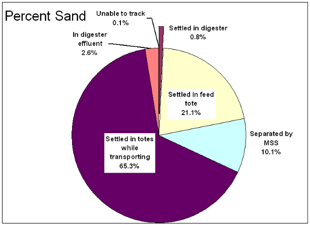
The pump reverser was tested, although it was found that the solids settling in the tank were not a significant problem over the operating period of the second Clarkson digester. This was largely due to the use of an external sand separator resulting in very little solids being introduced into the tank in the first place. The mass balance results of the sand separator trials are shown in Fig. 2.7, which clearly illustrates that the vast majority of sand is removed before the slurry is pumped into the digester tank [51]. The first version digester, designed by Mtarri / Varani LLC utilized this same feedstock directly and put 100% of the solids into the digester which contributed to the need for a pump reverser system.
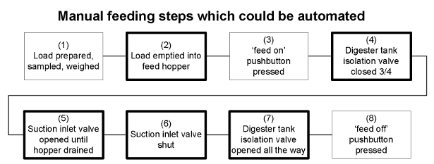
The manure system includes a feed hopper. In operation, the material to be fed to the digester was dumped into the feed hopper. Then, a “start feeding” push button was pressed on the control panel. This turned on the PLC’s feeding program, which performs mixing and electrical load control for the system. Once the pump was running, operators would operate two valves on the pump inlet side which forced the pump to suck from the feed hopper. Once feeding was complete, the feed valves were reset to their operating position, and the “stop feeding” button was pressed on the control panel, telling the PLC that feeding was complete and it could return to standard mixing and heating operations. The digester was normally fed approximately 20 gallons per day in two feedings, one in the morning and one at night. The feeding volume and times changed throughout the summer in response to data from the digester.
As the feeding was taking place, the effluent would be discharged through a three
inch transparent weir, sometimes also called an outlet box or goose neck. The height of
this device was set to maintain the appropriate pressure inside the tank which
was 8 inches of water (0.3 pounds per square inch). Adding material to the
tank caused an equal volume to be discharged through the goose neck. This
gravity discharge system worked well, with the lone exception of being one of
the remaining small-size fittings on the tank, requiring cleaning during the
summer.
inches of water (0.3 pounds per square inch). Adding material to the
tank caused an equal volume to be discharged through the goose neck. This
gravity discharge system worked well, with the lone exception of being one of
the remaining small-size fittings on the tank, requiring cleaning during the
summer.
Due to the fluid properties of manure, automatic feeding as low as 20 gallons through three inch pipe is very difficult to automatically meter effectively. Automatic feeding was further hampered due to the fact that the sand separation experiments required the mass of each volumetric feeding to be known precisely. Manure is highly non-homogeneous, and in order to get the reliable data for the system’s mass balance, each feeding had to be measured individually. Using buckets and scales, operators were able to measure volumes accurate to less than half a gallon and weights to less than 1 pound. Each feeding consisted of a filling gallon buckets from the raw slurry. These buckets were then weighed before being poured into the feed hopper, which was marked at the appropriate volume for that particular days feeding. Performing this task under automatic control would have required some mechanism able to measure both the mass and volume of a manure flow, while also being easy to interface with the system’s manure supply, which consisted of 250 gallon plastic tanks used to transport manure from as far as 70 miles.
Additionally, the experiments on which the digester was used required intermediate mixing and buffering stages to prepare various ratios of effluent, water, and manure for sand separator characterization. The equipment required to fully automate a sand-manure separator plant and digester are easily implemented on large scales with large flows and pumps where volume can overcome the manure handling issues and precise measurements of mass flow are not required.
The biogas handling system consists of the equipment required to safely remove the generated gas from the digester as it is formed. In a full scale system, the output from this system would feed into a prime mover or water heater through some kind of scrubber system. Due to the small scale of our system, the gas was flared or merely vented, depending on the flow rate of the gas. The small volume of gas produced by the Clarkson plant is not sufficient to even maintain a small flame on a Bunsen burner. Therefore, it was decided that not flaring the gas and merely venting did not pose a safety concern. However, on very large scale digester, producing 100’s of CFM of biogas, an improperly operating flare poses a potential safety risk.
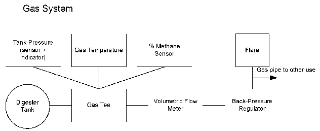
The digester gas system consists of a gas pipe leading from the top of the tank to the gas sense tee, through the volume meter, and then down a pipe to a combination back pressure regulator and water trap. The output from this then went to a flare, whose design was modified extensively by the manufacturer to accommodate our low flow situation.
The first several feet of pipe, and the all the gas instrumentation itself, was wrapped in heat tracing to prevent the biogas from condensing inside the instruments. The heater tracing should have been able to keep the heater tracing at a temperature far about the 37 C of the digester tank, although this was found to be difficult. Data indicates that the heater tracing gradually cooled off over time, despite the fact that energy was applied, and the tape was warm to the touch. The insulation over the heater tape was exposed to the environment, and any water which may have got between the gas piping and the insulation would greatly effect the heater tape’s ability to maintain the gas temperature. In addition, the top 3 inches of the tank itself were not insulated at all, to provide access to the bolts used to attach the lid. This happens to correspond to nearly 1/4 of the exposed gas area at the top of the tank. Therefore it seems plausible that the gas was in fact much cooler than the digester tank liquid, perhaps even enough to condense inside the gas piping directly over the top of the tank. This would have created a substantial additional heat demand which was beyond the capacity of the heater trace to provide.
These experiences have led to the understanding that a system based on cooling the gas may be a highly efficient and reliable way to remove damaging hydrogen sulfide from the digester gas stream. In winter, a sufficient temperature difference exists between the gas space in the digester and the outdoor temperature to condense most of the water out of the gas, which would take the water soluble hydrogen sulfide out as well. This may require a blower to increase the energy of the gas sufficiently to supply the engine of the generator set but is simpler and lower maintenance than other potential gas cleaning technologies.
The gas sense tee contained the tank pressure sensor, gas temperature thermocouple, and optical methane concentration sensor. The methane sensor in particular is very sensitive to both moisture and hydrogen sulfide, which is why keeping the gas from condensing was very important. The tee was plugged immediately into a standard bellows-type volumetric flow meter rated for natural gas service. This is the type of meter which is a standard piece of equipment on most houses with piped natural gas supplies. The meter is not designed for biogas service, due to hydrogen sulfide reacting with parts inside the meter, but it was decided that the meter, due to its low cost and very low pressure operation, was ideal for the length of operation planned. A full scale system would need to user a proper style of gas flow meter, or sufficiently clean and dry the gas to make a bellows-meter reliable. As part of this decision, the low flow of the gas system needed to be considered. Whereas a full scale digester could accurately measure flow using a turbine meter or other type, our low flow rates basically required a bellows-type meter, which accurately measure even the smallest of gas flow rates.
After the gas characterization equipment, the back pressure regulator was next. If a
generator was in place, this device would not be required, as some other gas pressure
regulator would maintain the tank pressure at its design point. Merely venting
the tank directly to the flare is not a valid idea, as sufficient positive pressure
must be maintained within the tank to maintain an anaerobic environment. In
the Clarkson system this pressure was 8 inches of water or 0.3 PSI (pounds
per square inch). Trials showed that six inches of water in the back pressure
regulator was sufficient to maintain the tank pressure at this design pressure.
The other two inches of water were taken up by pipe losses and the meter
itself.
inches of water or 0.3 PSI (pounds
per square inch). Trials showed that six inches of water in the back pressure
regulator was sufficient to maintain the tank pressure at this design pressure.
The other two inches of water were taken up by pipe losses and the meter
itself.
After the back pressure regulator, the gas was flared in a commercially available biogas flare, using a spark igniter. It was found that the gas flow was insufficient to support continual combustion. As such, flames were visible only during mixing and feeding operations, when the gas flow increased. Wind was otherwise sufficient to extinguish the flame, despite the flare’s wind covers.
The tank heater system consists of equipment and plumbing required to control the digester tanks temperature within appropriate bounds for the experiments being conducted. The heater system is capable of operation up to 50 C, although it was set to operate at 37 C for the duration of the summer’s experiments.
In the Mtarri / Varani digester, the heater system used a standard under-sink hot water tank and a very undersized pump. This pump was replaced with a generously oversized pump from a different project which was valved down to maintain the flow. The heat exchanger consisted of a stainless steel helical coil suspended from the lid. This configuration meant that a crane or hoist was required to remove the tank lid. Long rubber hoses were connected to this coil via tank top penetrations through a large number of various metal-to-plastic-to-metal threaded fittings. The fittings on the tank top were a continual source of frustration, as the rapid temperature cycling intrinsic in on-off heater control provoked these fittings develop leaks. The experiences with this system lead to lively debate and a vastly improved water heater system in version 2.
The version 2 Clarkson digester featured a stainless-steel flow through heater element and all soldered copper piping outside the tank. The heater fluid went through existing penetrations in the tank wall to flexible pipe segments feeding the existing helical coil. The helical coil was attached to stainless steel brackets welded to the inside of the tank. This not only allowed the tank lid to be managed by three people, but also meant that the tank, when open, could be easily entered and exited by standing on the coil support brackets. A properly sized heater pump was purchased based on pressure drop calculations and verified by measurements on the actual heater system.
The system is filled with a 50/50 glycol/water solution similar to that used in car engine coolant loops. The system was not drained for the winter upon completion of experiments. A recent inspection of the heater system after a typically rough and cold North Country New York winter showed that the heater loop has not leaked, and the system pressure is still at 3 PSI as it was when the system was taken out of service six months earlier.
The digester needed to be transportable, and as such was designed from day one to be carried on a trailer capable of being towed by a standard pickup truck. This required that the systems be not only reliable and robust from the point of view of weather and farm service, but also stable enough to be transported at highway speeds with a minimum of maintenance.
Additionally, it was found during the deployment of the original digester that access to the top of the tank and support systems was very important. The Version 2 digester features a support structure surrounding the tank that was designed to hold not just the plumbing and electrical enclosures, but also the weight of operators and equipment required for maintenance. A ladder was constructed to allow easy access to the top, and framing was constructed all the way around the tank to allow operators to reach valves and instruments without needing additional ladders or lifts. This system is illustrated graphically in Fig. 2.2.
Equipment access is of significant importance to digester maintenance. Due to the size of even the Clarkson digester’s modest 515 gallon tank, easily reaching the various thermocouple penetrations, valves, and gas systems is very important for system reliability. Human access to digester systems should be taken into consideration whenever possible, so as to avoid injury and time wasting disassembly and reassembly procedures.
The author assisted with the initial deployment of the first Clarkson anaerobic digester and participated in its operation and helped address various pumping and maintenance problems. The knowledge gained through this experience was applied to the construction of the second digester. The version 2 digester was designed predominantly by the author with the valuable assistance of Dan Valyou, Shaun Jones, and the Clarkson Biomass Group. The basic trailer and components of the original Mtarri / Varani design were re-used and the system was designed and constructed over a period of 12 weeks from December through February 2007-2008 with the dedicated assistance of members of the Clarkson Biomass Group and the support of the Clarkson machine shop.
The author analyzed shortcomings in the Mtarri / Varani digester, including deficiencies in the heating system, gas system, control system, and plumbing system and implemented solutions in the new version. Lessons learned in the engineering work that went into this design are described in more depth in Chapter 11.1. The Clarkson digester version two includes a state of the art local controller that is capable of being affordably upgraded to support real-time remote control capability, as described in Chapter 7.
Having a familiarity with the components of digesters from Chapter 2, this chapter will fill in the knowledge with an in-depth discussion of the local control system used on the Clarkson anaerobic digester. Having done that, an in-depth discussion of farm electrical loads and the impact of full-scale digester electrical systems on farm electrical service will be presented. These issues are all important to understand before an effective strategy of remote control can be developed in the coming chapters.
The time line of the development of this controller started as being a local controller for a system with a built-in bottom-mount sand removal system. This was the Version 1 digester, described earlier. Due to effort required to get the pilot plant mechanics operating, the controller wasn’t prepared in time for the initial installation on site, and all control functions were done by hand via front panel switches operating the AC contactors. During the trial period of the version one digester, the local controller was re-designed and further hardware ordered to meet the requirements of what was expected to be the version 2 digester. More thermocouples, more motors to operate on the various proposed sand separators, and more data channels. The ultimate goal of the Version 2 digester controller was to monitor nearly 40 temperatures around the tank as well as operate some kind of external sand separation equipment. This equipment was never constructed, and the equipment used in its place had its own on-board controller.
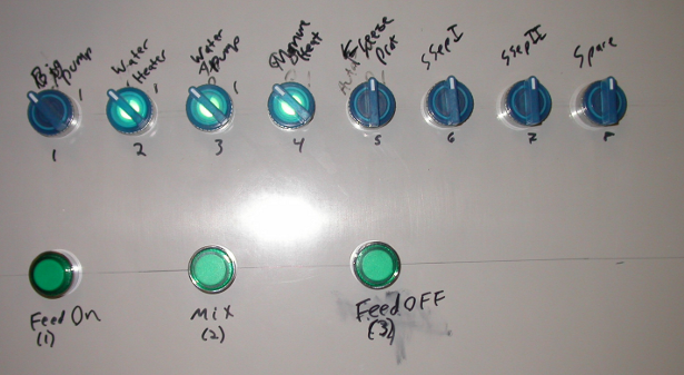
All the extra Input-Output (IO) equipment purchased for these goals was left unconnected. There are still contactors inside the AC enclosure with manual control switches labeled for use with a proposed sand separator design. After all of this, the goal was to deploy a web-interface for the digester enabling real-time control. This was not complete by the time the digester went on-line for the summer, although work has been moving in that direction. Discussions have been under way between the author and professors in the biomass group to complete the installation of a cellular data link over the summer based on the findings of this thesis.
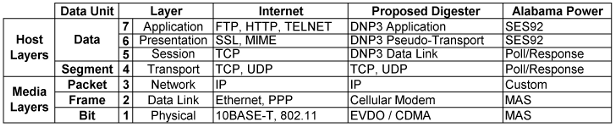
The addition of a more expensive firmware license to the current digester hardware will enable the digester to interface with on-line monitoring options available from various vendors, discussed in Chapter 7. Any vendor who offers a system which is capable of dealing with a Distributed Network Protocol Version 3.0 (DNP3) data stream, including those companies presented in section 11.8 are potential remote monitoring candidates. Future work to improve this controller will require a candidate familiar with various industrial control technologies, including DNP3 and the International Electrotechnical Commission (IEC) 61131-3 PLC programming specifications. In addition, knowledge of standard electric wiring practice and the Open Systems Interconnection (OSI) model for computer networks would be beneficial.
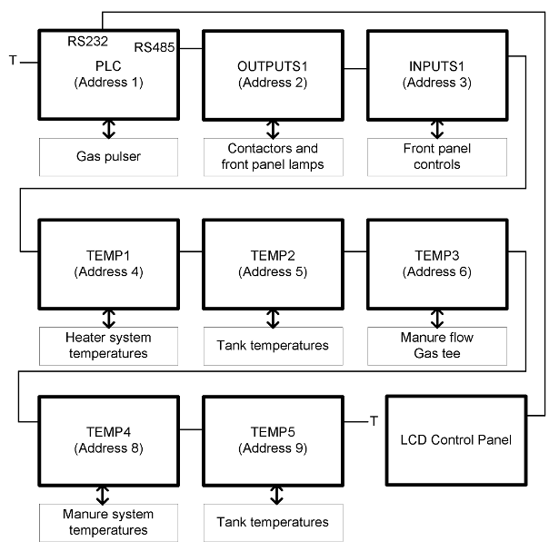
The digester’s control and DAQ system consists of a Programmable Logic Controller (PLC) and seven standard Input-Output (IO) modules connected locally over a daisy-chain RS-485 link. A daisy chain link is a standard wiring method in industrial systems, whereby the devices are plugged one into the next, often times with the wires coming from a device and going to the next device merely wrapped together and attached to the center device. This is illustrated graphically in Fig 3.1, which shows the RS-485 line going in a single path from the PLC through OUTPUTS1 and into INPUTS1. All the wiring for this signal is twisted-pair jacketed high quality cable. An LCD control panel is attached via a separate RS-232 connection to the PLC. All inter-device communications use the Modbus protocol.
Modbus was originally a trade name for the communications system developed by the inventor of the PLC, Modicon, in the late 1970’s. Since then it has become an open and freely available defacto communications standard, which is nearly ubiquitous on low-data rate sensing and control equipment. Modbus can be carried over a variety of electrical connections, including modern Ethernet TCP/IP connections. An excellent overview of the Modbus protocol is provided in [52].
In general, Modbus provides for coils, contacts, and analogs. A coil is analogous to a relay, and can be turned on and off. A contact is analogous to the contacts in a relay, and are turned on and off by other coils, or by external inputs. Analogs can be either read or written, and support various fixed point data forms depending on the type of analog value to be dealt with. A single Modbus system can have up to 256 devices, each device capable of having 9998 each of coils, contacts, analog ins, and analog outs. The digester channel list in section 11.6 shows all the Modbus addresses and channels. The SixNET column is used for mapping of Modbus channels to SixNET’s addressing system.
The main manure pump, for example, can be turned on by telling the Modbus representation of the coil with number 00009 at address #2 to energize, which in the hardware turns on a transistor which drives the contactor located in the AC cabinet, energizing the pump. A contact can be read, as is the case of the front panel switches, by reading the state of a virtual relay contact. Closing a front panel contact energizes a virtual Modbus coil which closes a virtual Modbus contact which is read by the software to tell the control program that the front panel switch has been closed.
Modbus was originally designed as a replacement for early automation systems. These early systems consisted of large boxes full of electromechanical relays and timers wired up to implement logic functions. Modbus was developed to enable people familiar with wiring large cascades of relays to easily replace those boxes of relays with easily reconfigurable controllers without substantial personnel re-training. The Modbus protocol when compared to modern industrial protocols like DNP3 seems very archaic because of these origins. However, because it relates obviously to physical relays, coils and other common industrial equipment it is a very popular and widely supported standard.
A Modbus compliant device enables reading and writing of coils, contacts, and analogs in a master-slave arrangement. The PLC forms the master of the digester controller, and all the other devices are slaves, forming “virtual IO” to the master station. This means that all the Input-Output (IO) modules in the digester, labeled in Fig. 3.1, are seen by the PLC as local input and output devices. The PLC, labeled as Address 1, when accessed via the Ethernet port looks like it has all the other channels of the other seven devices locally available. The goal of this topology originally was to make remote interfacing easier.
The PLC contains additional support for remote access over a different set of protocols, whereby having it appear as one large PLC with multiple inputs and outputs as opposed to multiple devices with their own inputs and outputs would be useful. The goal of the system was to be as integrated and simple to interface with as possible to the outside world. Describing this makes it seem more complex than it really is. In actual practice, the development of this kind of input-output system is easily handled in software packages available from the PLC’s manufacturers, literally as drag-and-drop or spreadsheet type interfaces. In the case of the Clarkson Digester, the software used to do the IO setup was the SixNET toolkit, available from the PLC’s manufacturer.
The actual amount of control and DAQ hardware installed on the pilot plant is in excess of what would ordinarily be required. The system has 40 analog instrumentation channels, 6 analog voltage input channels, 24 digital outputs, and 24 digital inputs. As presently implemented, less than half of all channels are actively utilized. This over design was due to changing design goals as the system progressed, while needing to be able to potentially control and monitor a sand separation and cleaning system. Additionally, the tank was originally specified to have three times as many thermocouples as were ultimately installed. The result of this is that the pilot plant has a controller capable of operating a very large digester, or an entirely integrated farm waste management system complete with remote web-based management.
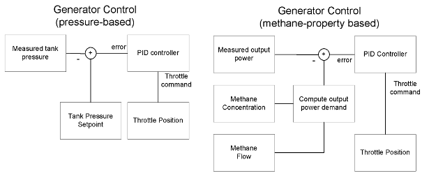
What follows is a discussion of each of the four blocks presented in Fig. 2.1 and what particular equipment and algorithms were implemented in their control. The four blocks are heater system, manure system, gas handling, and control. For purposes of this section, the control part of this view will cover issues relating to power monitoring, as the control system would need to be responsible for controlling not just the digester, but also the “gas use equipment”, which may have its own electrical interface. Each section discusses the system and its local control loop, and which variables of that loop would be essential for remote monitoring in order to effectively diagnose problems.
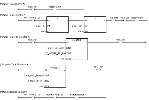
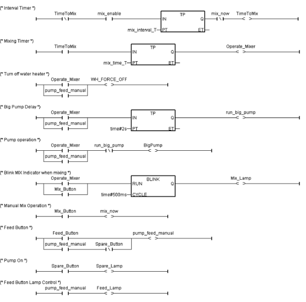
Pursuant to the goals of applying modern SCADA protocols to anaerobic digester control, the author implemented all control features in one of the languages defined by IEC 61131-3, known as Functional Block Diagrams (FBD). Due to the need present them full-size for readability, the FBD diagrams for the four key control aspects of the digester are presented in Section 11.7. In the sections which follow, these FBD diagrams are referred to when referencing the sections they control. The information contained in sections 11.6 and 11.7 constitute the majority of the details associated with the firmware of the digester. The program used to program the PLC was ISAGRAF Version 3.47, provided by SixNET for use with their hardware.
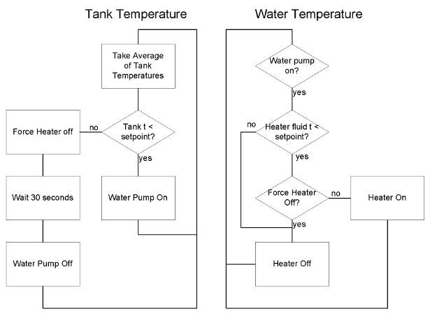
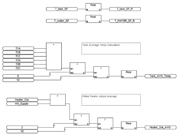
The heater element is a 240V flow-through unit rated at 4 kW. The control system consists of two different loops, one for maintaining the water temperature and one for maintaining the digester temperature. With electric flow through heaters, care needs to be taken to not over heat the water if the water is not flowing. For this system, the heater unit will not operate without the water pump being energized first, and if the water pump is de-energized, the heater shuts off. Control commands for the heater are generated by tank temperature averaging. All nine thermocouples submerged in the digester tank are averaged together, and that result is used to to determine the tank temperature.
The LCD interface contains a heater set point display, which allows for the user to set the maximum water temperature and the tank temperature. In operation, the flow-through heater element raised the water flowing through it an average of one degree Celsius. Trials were performed with the water not flowing and the heater on, and the 4 kW unit was capable of boiling the water in less then 2 minutes if the pump were to shut off. In a full size unit, the heater system may be of an entirely different design, perhaps piping the contents of the tank itself through an external heat exchange, instead of an in-tank spiral heat exchanger as used here. However, the basic system required to observe operation of the tank temperature control system are the same. The control system is illustrated in Figure 3.2, illustrates the two separate but coupled heater system control loops.
As currently implemented, there are four thermocouples in the heater loop itself, plus the “virtual” average-temperature reading thermocouple installed in the tank. Additionally, there is a turbine flow meter in the loop as well as two pressure indicators, on the suction and discharge of the heater system pump. An ideal design would include all of these devices automatically logged and recorded, however this is not necessary in order to establish if the system is operating correctly or not. The control loop in Figure 3.2 uses only the tank temperature and heater element outlet as its input variables. It therefore follows that these two data points are sufficient to tell of the heater loop is operating per specification. As will be presented in Chapter 5, a digester whose heater fails can be diagnosed by paying attention to various temperature variations, and complete monitoring of the multiple thermocouples as performed for this installation is not strictly necessary in a real world digester.
The heater system FBDs, presented in section 11.7 are HEATCON (section 11.7.2) and CALCTEMP (section 11.7.3).
The manure system plumbing is illustrated in Chapter 11Section 11.2. The manure system consists of one automatically controlled component, the five horsepower manure pump, and several manually operated valves. In the case of a full scale digester, these valves would be automated, or else separate pumps would be used, one for mixing, and one for feeding. The operation described here includes the processes which need to be manually performed, under the assumption they could be made automatic with only additional equipment. The controller design took this into consideration, and features extra open input and output terminals and AC contactors and relays for operating valves. Additionally, there are “hooks” in the control code to allow for easy automation of the valve commands.
The manure handling system is chiefly responsible for two key tasks on any digester. These are mixing the tank and feeding the tank. In some digesters, the mixing takes place as the system is fed, while in others, such as ours, they are distinct actions. It is important to the operation of a digester that the temperature be kept as uniform as possible within the tank. This is the goal of the tank mixing system. Some digesters, notably plug flow systems and lagoons, are unmixed, and therefore have simpler control needs than continuously-mixed type tanks. However, continuously mixed type tanks can be smaller and have shorter residence times, as well as increased gas production, due to the increased bacterial action that comes from mixing.
A significant limiting factor placed upon our digester was the available electrical service. More on this topic in Chapter 4. Our target farm had available only a single 30 Amp split-phase outlet with no neutral for powering our digester. This meant that we had 240 V AC available for use. A 5 HP pump, rated for 240V split phase service, requires about 23.5 amps full load, which is nearly the capacity of our available service.
The National Electrical Code (NEC) requires that proper motor starting equipment be installed rated for the full load current. This includes appropriately rated motor contactors, wire, and circuit breakers. Circuit breakers have a “curve”, which relates to the kind of equipment they are meant to protect. A breaker rated for starting a large induction motor, for example, will take longer to trip than one rated for computer equipment, as the induction motor will experience a large overcurrent each time it starts. Use of a circuit breaker rated for motor starting on a room full of computers may not adequately protect the wires in the room if a fault condition exists, and use of a computer room type circuit breaker on a large motor starting circuit would trip every time the motor was started, assuming the circuit breaker’s amp rating is the same in both cases.
The breakers at the farm were verified to be the appropriate curve, and a similar sized motor was running off this circuit originally operating a now-abandoned part of the farm’s manure scraper system. On startup, our manure pump consumed very nearly 23.5 amps, as was verified by measurements. The problem was how to keep the combined load of the heater system, control overhead, and other systems from exceeding the available electrical supply. In order to facilitate this, it was decided that the operation of the manure system would supercede the other equipment on the digester.
Therefore, whenever the system mixed or fed, the water heater and pump were deactivated to free up their current for use by the manure system. There has been interest in operating large digester loads during “off peak” electrical hours. However, this supposes that it is a good idea to operate all loads of a digester at the same time. In the case of the Clarkson digester, operating in this way would have more than doubled our peak load, from around 25 amps to nearly 60. On a large digester with 30 HP pumps, this could require electrical service for the digester increasing from 15 kVA, which is the max of the single large pump and other small control loads, to 30 kVA or more. As a general reference, 24 kVA is about the same size as a standard domestic home electrical service.
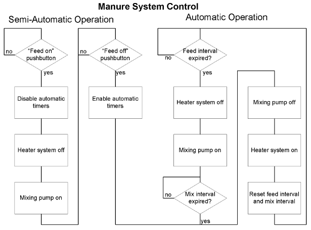
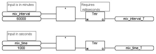
The basic control loop of the manure handling system is illustrated in Figure 3.3. This figure illustrates the effect of “semi-automatic operation”, which was what was performed for feeding, and “automatic operation”, which is how the system operated unless the Feed On push button was operated. The feed interval and mix interval were entered into the system via the LCD control interface by the operator filling in the sentence “Mix tank every xxx minutes for yyy seconds”, where valid ranges for xxx and yyy were from 0 to 1024. This setting was changed over the summer, to compensate for various feeding schedules.
It was learned through operation of the summer that counters are needed as well. In order to ascertain if the feeding schedule is proceeding as planned, and that equipment is running as it should, the total pump run time and number of pump cycles performed under manual control needs to be recorded. Having a running tally of total pump run time plus number of pump start and stops would have made load calculation much easier. In addition, keeping track of total pump run time is essential for planning maintenance on rotating equipment like pumps, whose maintenance and lubrication intervals are typically specified in terms of hours of operation.
In addition to the control flow illustrated in Figure 3.3 there were also manual operations required to operate valves to feed the system. This was why the semi-automatic feeding operating was installed. As the system went through its design phases, originally it was planned to automatically feed from some storage vessel or hopper. Making the feeding fully automatic is easy from the control, but very difficult from the balance of plant and cost point of view for the size of the pilot plant. Adding automatic feeding would have required an extra pump, or automatic valves, which in itself would have been doable. What made it impossible was the need to characterize flows and mass balance for the sand separation experiments taking place. Metering sand density, mass, and other parameters, while also taking samples for lab analysis, is far beyond the scope of what would be required for commercial operation of a farm-based digester. However, the manner the system was fed was still valid, and could be employed instead of using a separate pump to feed the tank.
Figure 3.4 illustrates the steps to feed the tank. The feed hopper is a 20 gallon capacity plastic cone-bottom vessel which was attached to the manure pump suction line. The steps in the bold boxes in Figure 3.4 could be automated, using the control hardware already on hand, with the addition of automatic valves. The benefit of using this system is that only one pump is needed for mixing and feeding, with the additional expense of two automatic valves. The suction inlet valve and tank isolation valve need to be made motorized in order for this style of feeding to work automatically. Consult the plumbing diagram in section 11.2 for understanding of these valves in the manure system. It may make more sense for many designs to use a separate pump for feeding the manure, as it requires no additional valving.
Automatic valves come with feedback elements, such as variable resistors or micro switches, which indicate if the valve is closed, open, or in-between. These devices work to verify the valve’s operation. In practice, valves in manure service are highly unreliable devices due to the very rough nature of sand laden dairy manure. Various farmers report having to replace their large manure pumps every 18 months as a result of sand damage, and valves suffer the same fate. Automatic valves, in that they depend on electric or pneumatic means for operation, may have another shortcoming when applied to sand laden dairy manure: They can seize up. Whereas a manual valve can be “worked” back and forth by hand, implementing that feature in automatically controlled valves is very difficult. If it is a choice between automatic valves and separate pumps for mixing and feeding, separate pumps should be chosen, due to these issues.
The last feature of the manure system, which was not automated, was the pump flow reverser, a series of four valves which enabled the flow of the pump to be changed in direction. Normally, the flow within the digester tank is from the bottom to the top, counterclockwise in the plumbing diagram. Operating the pump reverser causes the flow to suck from the top of the tank and return through the bottom, clockwise in the plumbing diagram. This system was designed to remove sediment buildup by enabling the tank contents to be fluidized for draining. This principle is not necessarily applicable to large-scale digesters, however, due to their having much larger tanks, making fluidization much more difficult. As a means to cure pipe clogs and break up floating tank top scum it appeared to be successful.
The manure system FBDs, CALCMIX and MIXCON, presented in sections 11.7.1 and 11.7.4 respectively show how these features were implemented in a standard IEC 61131-3 compliant manner.
The gas handling system on the Clarkson digester is fairly simple in function. The goal is to conduct the gas away from the top of the digester to a flare while still maintaining the design pressure of 8 inches of water within the tank. Anaerobic digesters need to operate at some kind of positive pressure above local atmospheric in order to prevent ingress of atmospheric oxygen. The gas system implements several instruments to measure the gas properties. The hardware of the gas handling system covered by this section is diagrammed in Figure 3.5.
The gas first leaves the digester tank, and flows through the “gas tee”, which is a metal pipe tee to which the gas characterization hardware is attached. This includes a tank pressure sensor and manual readout gage, a thermocouple for temperature, and a optical methane gas concentration measurement instrument (BlueSens BCP-CH4). The gas then flows through a bellows type gas flow meter familiar to most as the standard home gas meter (American Meter AC-250). Finally, the gas flows through a back-pressure regulator. If the gas were to be used for something else, it is after the back pressure regulator that it would be diverted to go to running a generator or firing a water heater. In this case, the gas is simply set afire by the flare.
The components of the gas handling system as implemented here are the minimum required to provide what is necessary for control and remote data access. Such information is required for generator or water heater control to optimize power produced from the equipment.
There also needs to be some kind of pressure regulating device. This could be a gas bubbler, as is installed here, or something more complex. More complex could be a gas storage tank and compressor system coupled to an engine, or a floating top to act as a pressure regulator instead.
Generators and water heaters are normally operated on continuous gas supplies, sufficient to maintain their operation when called on. Standard home piped gas service, for example, is expected to always operate when the furnace is called to provide heat. In a digester, this may not be the case. Depending on feeding rate, tank temperature, material to feed, and amount of mixing, both the gas flow rate and the methane concentration can fluctuate considerably. In order to accommodate this, either gas storage needs to be designed into the system with some kind of variable-volume cover, or else the gas use device must be controlled to never totally empty the tank of gas. Such a failure would not cause permanent damage to the system, but would cause intermittent and annoying generator issues and may increase maintenance costs. See Chapter 5 for more information on this topic.
During mixing cycles, when the material was agitated, enough gas was produced to keep the flare lit for the duration of the mixing interval. This suggests that even on a large-scale tank, the generator output may need to be increased during tank mixing cycles to use the extra gas produced and avoid flaring or tank pressure increases.
Full scale digesters either need to operate with engine load dependent on gas production, or have sufficient gas storage to even out the digester gas production. The cheaper option would be to control generator output based on gas, but that may not allow the system owners to generate electricity during the peak times when the economic conditions are best. This problem is compounded by the additional use of digester gas for the heating of certain kinds of digesters, which means there is a three way balance to solve. Work has gone into solving this problem by researchers in Clarkson University’s Biomass group, notably Yotam Weldetnsae who used computer simulation to analyze the best way to share biogas between water heaters and generators, including economic concerns and net metering [53]. Being aware of these problems means that the control system can partially accommodate some of the difficulties associated with this control. For the initial version of the digester, no attempt was made to do anything with the output from the gas measuring instruments aside from simply logging them.
Two potential control loops for generator control are demonstrated in Figure 3.6. In the pressure based algorithm, at left, the tank pressure is measured and compared to the tank pressure setpoint to change engine output power based on tank pressure. The methane-property based loop uses methane concentration and methane flow to adjust engine output power based on computing the actual maximum power output available for the current mix of gasses combing out of the digester. In reality, a system utilizing both technologies may be best, if the sensing requirements could be met. If a water heater is also installed to use part of the biogas for heat the generator load problem becomes more complicated. This would require a more complex digester control algorithm which would need to manage the operation of all the equipment requiring digester gas for operation.
There are 46 channels associated with operation of the Clarkson digester. To improve readability the table explaining the details of all 46 points is omitted from the text, instead being included in section 11.6. A full scale digester would have a similar set of points to monitor, although of different types. The Sheland Farms digester monitors only 17 points, presented in Fig. 6.1. However, the Sheland digester has many channels relating to power use, whereas the Clarkson digester has many extra temperatures which are not measured in the Sheland plant. Furthermore, the Clarkson unit has its pumps under the control of the local controller, whereas the Sheland unit has all pumps operated by manual timers on the pump starting electronics. For a full discussion of channel requirements and data needs, see Chapter 7.
The local operator interface needs to the ability to view the measured values of all the sensors and configure key operational parameters. Additionally, the local operator interface needs to provide the capability to control pumps and contactors under manual emergency control, for when the automatic controller is offline or manual testing needs to take place.
The way chosen to implement local control interaction for the Clarkson digester was a small and inexpensive touch-screen LCD device from an industrial controls supply house. Other digesters seen use standard electric rotating timers, the kind used for automatic lighting control in homes, or even farmers operating switches to run equipment. The Human Machine Interface (HMI) device, illustrated in Figure 3.7 features a touch-screen section approximately three inches by two inches, and a membrane keypad for numeric entry. The HMI itself was mounted on a swing-out panel inside a lockable transparent weatherproof enclosure. Behind the swing-out panel is the wiring for the RS-485 loop and DC electrical and sense connections.
The author designed a programmed a hierarchical menu system for interfacing with the digester, showing all key parameters in real-time as well as allowing setpoints to be programmed through the display. The author produced an instruction manual for the operation of the digester which was primarily intended for internal use by the group, but us available for download from [54]. All setpoints are stored in non-volatile memory enabling the digester controller to return to standard operations after power failures. The menu structure is illustrated in Figure 3.8. The color of the LCD screen’s backlight is programmable by the PLC, alerting the user via its color as to the status of the command. Green screens are informative, and touching the screen does nothing. Red screens are control screens, and operating their controls can energize equipment and change settings.
Most of the screens of the HMI are informative. Upon initial powerup, the digester’s firmware version is displayed. Pressing anywhere in the screen brings up the main menu, which consists of “control, params, tank temps, overview”. The overview button displays all immediately valuable operating parameters, including tank pressure, gas concentration and pressure, and pump status and temperatures. The Tank Temps button shows a real-time view of the current temperatures reported by all nine in-tank thermocouples. This is especially helpful when troubleshooting and replacing thermocouples. The “params” option opens up a parameters screen, where options are available to adjust temperatures and mixing times. The control option opens up another menu screen, which allows operators to view current contactor status (engaged or disengaged), as well as simple diagrams showing all measured parameters.
These simple diagrams include the water heater system, with all thermocouple temperatures shown on a schematic of the heating loop. There are also similar schematic views of the gas system and manure system. Every tank measured parameter in the system is available somehow via this local control screen, and an effort was made to make it easy to navigate and obvious to use. The ultimate goal is to enable a service person unfamiliar with this particular digester, but having familiarity with digesters in general, would be able to adequately troubleshoot the equipment using information from the HMI.
On a full scale digester using this kind of controller, the same HMI would be used to display generator status and water heater status, so long as those devices could interface via compatible control interfaces. The goal of using the LCD panel with the Clarkson Digester was to showcase the ability of standard industrial control parts to be adapted to digesters, as well as providing one point of interfacing for all digester equipment to simplify operating instructions and equipment maintenance.
Should some catastrophic outage occur which damages the entire control system, all local control systems have manual control which can operate the systems as locally as required. The digester controller discussed here contains front panel control controls mounted on the front of the AC control cabinet as illustrated in Fig. 3.9. These switches are capable of being set in one of three positions: “On, Off, and Auto”. In “on” the contactor is directly energized and the pump or system will run. In “off” the control wire from the power source is physically disconnected, and no operation of the device is possible. This would be combined with turning off and locking out the disconnect switch or circuit breaker for maintenance of a full size system. “Auto” is the standard operating position, and connects the contactor’s control lead to the PLC input output system.
In addition, these switches are illuminated, so that when the circuit is energized, the lamp on the control panel glows. In Fig. 3.9 the four top controls are pointed to the left, which is auto, whereas the right hand four controls are located in the center, which is off. The controls labeled 2,3,4 are energized in the picture, as shown by the fact that they are illuminated. The bottom row of buttons controls the semi-automatic features of feeding and mixing.
This chapter describes the local control system designed for version 2 of the Clarkson digester. The decision to use standard IEC 61131-3 compliant languages and industrial communications protocols was made by the author, in preference over a custom-designed MatLab/Simulink script and associated IO hardware. This controller took shape from design notes originally made by Prof. Eric Thacher. The choice to use standard hardware and software approaches allowed the Clarkson digester to be assembled and tested rapidly, and the author’s derived flow through heater control loops and mixing programs to be implemented with ease.
The system as constructed took advantage of standard industrial control wiring practices and enclosure types for a rugged, weatherproof solution. The human machine interface, both the manual control panel and the LCD and membrane-key HMI equipment, was designed and constructed by the author to maximize the ease of local control, while simultaneously providing the basis for remote system control as described in Chapter 7.
Of interest to farmers considering the installation of anaerobic digesters is how the digester will effect the electrical systems on the farm. Farms tend to be located in rural areas. Power distribution in rural areas tends to be a radial system, where one set of wires runs out from a central substation, often times along the roads that serve an area, with multiple “service drops” to each customer along the line [55]. These systems are the least reliable as a fault along the line will interrupt service to all customers downstream of the fault. In order to address this, primary loop systems can be used, whereby the local distribution line is connected to substations at both ends. Large cities and very dense population centers have have electrical feeders in a grid pattern below the streets, allowing for many switching options to keep customers served during outages and maintenance work. Operating such systems is very expensive with substantial initial capital costs.
Because of the large geographic area covered, rural utility customers are served by the simpler and less reliable radial system [56]. Each distribution line will run along a street and serve multiple homes or farms through a local step down transformer at 240 Volts located near that particular customer. This 240 Volt service is the same as that provided to the vast majority of residential power customers, and is called “split-phase” service, to differentiate it from “three-phase” service. Split phase service provides two legs of 120V which can be combined for 240V to supply larger loads such as clothes dryers and large pumps.
Large commercial customers and more densely populated areas will be served by three phase electrical service. Three phase electrical service is common for commercial and industrial buildings, and can provide 208, 240, or 120 volts depending on how it is wired at the service drop. Due to the loads encountered on large scale dairy operations, the installation of digester equipment may move their electrical requirements into the commercial or small industrial range, therefore requiring the farmer to upgrade the electrical service to three phase to meet the utility reliability requirements. This could be a substantial cost, depending on how far the farm is from the nearest 3-phase distribution infrastructure.
Much of the work by Clarkson University has been performed in reference to the North Harbor Dairy in Watertown, New York. There have been several analyses performed on this dairy relating to farm electrical loads and power bills, including an in-depth analysis of using three-phase generators on single phase service by Masemola [57], and an exploration of system optimization by Weldetnsae mentioned previously. Part of Weldetnsae’s system optimization is based on operating assumptions relating to how often pumps and equipment would operate on the digester. His research demonstrates that there is a relationship between electrical load of the digester systems and optimal gas sharing between heat and electrical power generation.
Here will be developed a method to ascertain the actual total power use and run time of all individual systems on the pilot-scale digester, broken up in terms of the four standard operational digester blocks (Heating, Manure Handling, Gas, and Control). The load figures from this chapter, as well as those from Chapter 6 can be used to benchmark other digester designs and their impact on local farm electrical systems.
The Clarkson Anaerobic Digester was operated for three months in the summer of 2008. Through the last 34 days of operation, the digester had an integrating kilowatt-hour meter installed to log energy supplied to the digester. This logger was installed on the main supply for the power going to the site where the digester was installed, so it also measured additional loads relating to the sand separation system and other random loads. However, these loads were not very large, and were operated for a very small fraction of the time that the logger was installed.
The data logger took a sample every one minute of Kilowatts (kW), Kilovoltamps (kVA), Kilowatt-hours (kWh), Volts (V), and Amps (I). The power logger system was totally independent of the rest of the digester controller. Originally, it was planned to have a power meter installed on the system to monitor power use of the system, but it was not in place at the start of the summer’s operational period. The fact that the power logger was a separate stand alone device created problems for the reliable gathering of data.
It was thought that by storing power values every minute there would be an accurate record of all the power use by the system. This is partially true. The power logger accurately measured all the power, but when comparing the electrical data to the digester control system, accurately figuring out which device was using which power was very difficult. The two systems were not synchronized, and as such, numerous effects show up as data sampling errors. Any future digester system needs to integrate the power logging functions into the rest of the DAQ and Control equipment, to provide a useful accurate real-time record, without the need for the significant post-processing discussed below. Additionally, run-time counters will be installed in the future versions of the digester, which will report on various devices run time. This can be used for power calculation or routine maintenance requirements. This same sample time skew issues shows up in Chapter 6 when discussing failure modes and power use of the Sheland Farms digester.
In order to extract the actual true power use for each of the sections in the controller, a fair amount of analysis needs to be performed. The horizontal axis for most of the graphs in this chapter are time, in minutes, from the first operation of the power logger. The vertical axis of most graphs are power in kilowatts (kW). To get a feel for what the raw data looks like, consider Figure 4.1. Notice that the time goes up to 50,000 (there are actually 49,940 data points in the figure). Additionally, observe that it looks like white noise, with some vaguely apparent bands crossing diagonally. Each point in the graph represents the power, in kilowatts, averaged over that particular minute. Voltage and current were measured as well, but are not analyzed.
The most obvious manner to analyze the data would be to attempt to line up the data using time, and then assume that each device’s power consumed was the amount consumed while the time lines up between the two data streams. That method, however, would not be accurate for the following reasons.
For these reasons, and others, it was chosen to analyze the data entirely from the power point of view. Figure 4.1 is the kind of data retrieved from using timed sampling of power values with highly intermittent loads. If one were to average out several dozen or a hundred digesters using the same kind of control technology, the average load of that whole system would converge to a set of points forming a line with an approximate load of around 2 kW.
All graphs and sorting in this process were carried out using Mathematica Version 6.0, and complete code is included in section ??.
In order to separate the data into its individual parts, knowledge of the initial equipment is required. For instance, the quiescent load of the control hardware is known from notes taken during construction and presented here in Table 4.1. Additionally, it is known how much heater tape is installed on which circuit, and the approximate behavior of the large pump. In going through the following analysis, each step’s assumptions and loads are presented as well as discussion of the remaining amount of power to be accounted for.
Recall our idealized digester consists of four key systems: heater system, manure system, gas handling, and control. For the purposes of the power analysis, we will consider the following for loads:
Ptotal=PWaterHeater+PHeaterTape+PControlOverhead+PManurePump (4.2)
In Eqn. 4.2 PWaterHeater refers to the total operating power required for the water heating system, including the circulation pump. PHeaterTape refers to the heater tracing applied to the gas system and manure heater sections. PControlOverhead refers to the control system overhead, and PManurePump refers to the power used by our manure handling system. At the end of this chapter, a table and charts will be provided dividing up the power according to our idealized digester block description. Additionally, the computed total powers will be divided by days and averaged into energy at the end of the chapter.
It is important to realize that through the following sections, care is taken to maintain the time dependency of the data. The power logger file contains the power averaged over each minute of system operation. The only way to effectively remove power time skew is to find the total device power use by processing the individual average powers per minute, and then summing and dividing to convert to energy use.
The easiest load to compute is that of the control system. It is a small fixed load whose operating power requirements were measured and agree well with the documented electrical data for the equipment. In order to provide worst-case analysis, it is assumed that the control system is operating continuously at its rated electrical consumption. Table 4.1 shows the equipment in the control system and each component’s rated DC power draw. With a power supply efficiency of 75%, that translates to 30 watts continuously drawn for the operation of the control system.
Notice that there is no included numbers for the DC contactors. The DC coils are 24 Volts, 100 mA per coil when energized. However, because the duty cycle of the contactor coils is so very small, it was decided that this power could be omitted from the study. However, this may not be the case on a larger digester, where far larger motor starters are required. It will be shown that the digester control overhead is a very small part of the overall system’s power use.
| |||||||||||||||||||||||||||||||||||||||||||||||||||||||||||||||||||||||||||||||||||||||||||||||||||||||||||||||
Subtracting PControlOverhead from the raw total power data shown in Figure 4.1 essentially moves all the data down 30 watts, which is very difficult to see on a graph of with a 4 kW vertical scale, and has therefore been omitted.
Premaining=PWaterHeater+PHeaterTape+PManurePump (4.2.1)
Heater tape, sometimes called heater trace, is a self-regulating polymer embedded with two conductors. The material changes its resistivity, and therefore its thermal output, according to prevailing temperature conditions. The heater tape was always energized, and although its load changed with temperature, the variance would have been very small once the system heated up. Examining the data PRemainingfrom the previous section, it can be seen that 370 watts continuous load is what remains of the baseload power consumption. The only devices permanently on and attached to the AC mains were the control system and heater tape. All other loads were switched according to the control algorithms described in Chapter 2. Setting an upper bound of 370 watts, the heater tape power consumption can be deduced.
Taking into account the amount of heater tape used and the different power levels of tape applied, the difference in power used for the manure heater system and the gas heater system can be further divided. At the time of the installation, around 100 feet of heater tape was installed. Approximately 25 feet of this tape was used on the gas system, and 75 feet of tape was used on the manure heater system. This knowledge allows us to subdivide this load into two categories for final evaluation, as demonstrated by the conclusions section of this chapter.
The power equation now looks like:
Premaining=PWaterHeater+PManurePump (4.2.2)
The next thing to do is to separate out the load used for the water heater and the load of the manure pump.
Initially, separating pumping power from heater system power was attempted using the water temperature inlet and outlet temperatures to compute the duty cycle of the water system. However, this yielded a fluid pumping power which was far less than what would be required simply by dead-reckoning pumping power based on average pump run time computed from the pump duty cycle settings in the menu screen. It was therefore decided to examine the electrical loading of the equipment directly. A similar attempt was made using power factor to determine pump operation time, but this produced unreliable results because the heater pump had its own transformer, and therefore contributed to power factor variation as well.
The controller on the Clarkson digester was programmed to allow only one large load to be operable at a time, either the heater system or the big pump. By design, therefore, when the manure pump is turned on, the heater system is turned off. With this understanding, the operating power of the pump can be figured out from Premaining.
Although the actual run time of the pumps are not known exactly, an estimate of the run time based on digester operating parameters can be used to set the cutoff power factor to figure out the total power of the pump. During the entire 49,940 minutes that the power logger was installed, the digester was set to operate the mixing pump for one minute every 29 minutes. The result of this is that the pump would run for one minute every half hour. That would be approximately 1665 minutes worth of pump run time. However, there is also the time spent feeding the tank. The semi-automatic feeding procedure re-sets the pump timing interval. This may add an extra few minutes run time per day, depending on when in the automatic cycle the feeding was performed. On average, we can assume it may add an additional half minute per day, for another 18 minutes of run time. Therefore, the total pump run time should be approximately 1683 minutes out of the 49,940 minutes the power logger was installed.
Furthermore, the heater system load is known with some degree of accuracy. During testing, it was found that the heater system and pump consumes 2.8 kW when operating at around its operating temperature of 37 C. What is unknown is the exact time the heater element operated. These two pieces of information can be combined to form a solid understanding of the total pumping power. In summary, the heater system operates with a 2.8 kW load, and the pump operated for approximately 1683 minutes. Of course, there would be some minutes that power was shared between pumping and heating. Looking at Figure 4.2, a graph of Premaining, sorted in order of power use, and zoomed up to the area of interest, a transition period between minutes 42,000 and 48,800 is clearly visible. Using our constraints of run time and power, and deciding on a maximum power based on Figure 4.2, it seems plausible to assume that the power consumed greater than 2.75 kW would be for the pump. This then allows the data to be sorted in time order, and subtracted from Premaining, to yield the actual pumping power over time.
It stands to reason the the only remaining category not yet accounted for in our original power equation is PWaterHeater. Therefore, PWaterHeater is all that remains after subtracting the other three loads from Ptotal.
So far show we have found the time-of-use average power for each of our four use categories. In order to appreciate the meaning of this from a system scaling and farm load point of view, this information needs to be related to something of more standard usefulness in billing and discussion: the kilowatt-hour (kWh). This is the amount of energy consumed when one kilowatt (kW) is utilized for a time of one hour. Most electric bills for small businesses, commerce, and residential areas are billed in this unit, as it provides an easy way to talk about energy use for a day or a month, or average energy use over a period. This is very important, given the noisy nature of the graphs in the previous few sections.
There are several ways to get kilowatt-hours from the data set. Perhaps the most obvious would be to take the time a pump was running, and multiply it by the average electrical load of that device. This is a standard idea when discussing equipment, and could be applied here, for sake of example. Recall that the pump was operated for 1683 minutes, or 28.05 hours. Measurements taken indicate that the pump, when running at 208 volts, used around 23 amps to mix the tank at a power factor of 0.86. Therefore, total power use is 4.114 kW. The total energy use of the pump for the duration of the test should be 28.05 x 4.114, or 115.4 kWh. This in is nearly twice the actual energy use, when computed using the method described below. This is because the pump does not always run for the full minute each and every minute. This is why such length was gone through to try and maintain time in the previous discussions.
The most appropriate way to calculate total energy use is to do a discrete-time summation over the entire sampled data space of all 49,940 points of power data available. Power is the amount of energy used per unit time, as follows:
Paverage =  ∫
t2t1P(t)dt =
∫
t2t1P(t)dt =  (4.2.5)
However, because the time intervals of the logger were always exactly one
minute,  = 1 and △t12 = 1. This allows equation 4.2.5 to simplify down
to:
= 1 and △t12 = 1. This allows equation 4.2.5 to simplify down
to:
Paverage =  (4.2.6)
for each one minute sample. Applying units to equation 4.2.6:
Energy = PAveragex1.0 (kW ∙min) (4.2.7)
Equation 4.2.7 is only valid for the case where minutes equals one, which is the case for the power logger as installed. This gives the rather odd unit of energy as the kilowatt minute, as opposed to the kilowatt hour. It also gives the unique result that the energy (in kilowatt-minutes) is numerically equal to the average power logged over that minute. Thus, to find the total energy used by a device, sixty of the average one minute power samples, which are really energy values in kilowatt-minutes, can be summed up and divided by sixty minutes per hour:
Energy(kW ∙Min)× =Energy (kW ∙hour) (4.2.8)
Therefore, by combining the power logger’s averaging of power over one minute and storing it every second allows the total energy to be found (in kilowatt-minutes), just by summing up all the single-minute samples and then dividing the total by 60 to get kilowatt-hours (kWh). This method of using energy into power is only valid because of the enforced one minute regular sample intervals. Using this method with samples having variable time intervals would be ineffective.
This method was applied to each individual load to populate Table 4.3. This was possible because of the effort to maintain the one-minute sample interval time information of the previous sections.
Using Mathematica’s built in functions, all the kilowatt-minutes were summed up according to their individual operating times to give total energy per device in kWh over the total time the logger operated. If the kWh per day of a device was required, as was the case to populate Table 4.2, then only a days worth of minutes (1440) were summed up instead of all 49,940. This method was experimentally validated by comparing the method described above to the total energy (in kWh) stored by the power logger. According to the power logger, the total energy used over the course of the operational period to which the digester had its power logged was 646 kWh. Using the methods outlined in this chapter, and summing all the individual loads together, the total power use was computed to be 641.58 kWh, a difference of less than 1%.
If the power use is extrapolated out over the entire summer, rather than just the portion during which power was logged, the total energy required would be 1687 kWh, for a cost of $202.44 at $0.12 per kWh. The summer power requirements, divided by load are summarized in Table 4.2. The digester had a power logger installed for 34.68 days, out of a total operational period of 91.18 days. The average electricity price was taken to be $0.12 per kWh. In addition the table contains a column for a new measure, electro-hydro efficiency, which is the ratio of watt-hours per gallon day of digester operation. The unit’s total hydraulic volume is 515 gallons, and it’s operating time was 91.18 days. The smaller this number, the better the system is at utilizing its energy.
|
The Sheland Farms digester covered in Chapter 6, with a tank capacity of 160,000 gallons and an average daily load of 14 kWh has an electro-hydro efficiency of 0.0875. The Clarkson digester looks quite bad by comparison, unless it is considered that the results of Table 4.2 include using electricity for heating. If some other means could be found to heat the Clarkson pilot plant, then its electro-hydro efficiency would improve to 5.5. in general, the larger the tank volume for the same size of pumps, the smaller and therefore better the electro-hydro efficiency would be. A design proposed for the North Harbor Dairy by Stearns and Wheler LLC shows an average daily load of 892 kWh per day and a tank volume of 240,000 [58]. This would provide an electro-hydro efficiency of 3.71.
Of note here is the amount of energy consumed by the manure heater. The original design goal for this was to compensate for the ambient-temperature manure in the plumbing system dropping the tank temperature by heating and insulating a section of tank-external manure volume. The large electrical load that this heater tracing required suggests that the heater tape may not be the best solution. It is important to recall that any manure pumped outside the tank will gradually cool, as the plumbing system is largely uninsulated.
The average daily energy use, divided by use area in a pie chart, is presented in Figure 4.3. In the case of the Clarkson Digester, the volume of liquid in the plumbing not within the insulated tank amounts to 9% of the total system volume. A farm-scale digester would have larger pipes and pumps, but a much larger tank, perhaps removing the requirement for this kind of manure pipe-heater system. However, a larger digester tank would also necessarily be moving much large flows through the plumbing, further complicating heat loss through pipes. Given the electrical requirements of heater trace, and the detrimental effect of cool manure on digester operation, digester plumbing needs to be kept indoors and insulated, if possible.
This chapter describes the method used to process raw minute-by-minute power data from a logger installed on the pilot plant into total energy use and operating cost, organized by area of interest. This chapter also demonstrates the complex procedures required for ascertaining useful power data from such a non-integrated power logging device. Fully integrating a power meter into the rest of the control system, and using it to report actual power and energy values as requested by a remote system, would provide a much larger benefit to digester maintenance than the methods described in this chapter.
During the operational period of the digester over the summer of 2008 numerous experiments relating to sand studies were performed. Also during this period numerous failures occurred due to random events, equipment vandalism, and operator error. When a minor problem developed or a system failed, no one was immediately notified and no repair action could take place until the next feeding crew was able to manually check the status. Even then in many cases problems were missed due to lack of reliable on-site trend analysis.
With the current digester controller and indeed many other renewable energy control systems data is gathered once a day or less frequently to diagnose long term problems. What follows are five examples of real-world summer situations where a more immediate data connection would have been very useful because systems operated sub-optimally and required rapid outside intervention.
The importance of the event is discussed, as well as the reasoning behind the needs to be able to see the events in real-time, and the monitored channel required to identify the event, as well as a discussion of the reporting frequency required to discover the fault before it becomes a major concern.
Figure 5.1 illustrates the tank pressure and methane flow rate versus time. The methane flow rate associated with this scale of digester is very small, but none the less indicative of a larger system. The digester at its peak produced more than 80 cubic feet per day. The bottom line of the figure shows gas production in cubic feet per day. The top line of the figure shows tank pressure. Of particular interest in this section is the peak of gas production at around 450 hours of operation. Knowledge of the flow rate on a tighter time schedule would have allowed the system operators to make more informed decisions about the feeding rate for the tank, allowing for continuously sustained gas output.
Monitoring gas output in real-time is essential to efficient operation of anaerobic digesters with generator plants, as the gas output is used to power the generator itself. Knowledge of a fall in gas output or change in methane content could signal that the generator may not be able to operate at peak capacity, or in fact that the generator loading has to change to maintain tank pressure. Unless gas storage is provided, the generator output needs to be controlled according to gas flow rate and tank pressure.
Of further interest in Fig. 5.1 is the tank pressure. The top line shows tank pressure as a function of time. Notice the steady upward trend in this line and the large dips. Each large dip corresponds to a loss of pressure in the tank which would be an emergency situation. Such a large drop would be caused by a rapid release of biogas due to a valve opening or even something as catastrophic as tank seam failure. With a real-time data acquisition system, the flow rate could have been adjusted at around 450 hours to maintain peak methane production.
In this particular digester, the rapid dips in gas pressure were due to valves being opened, typically when work was performed on the gas measurement system. Upon further inspection, the gradual rise in gas pressure was in fact not measurement error, but seemed to have been caused by a buildup of a growth in the flame-arrestor of the gas flare.
In order to use gas production as a means to judge feeding rate, the output needs to be logged at least on a daily basis. However, the local control system would need to know the gas parameters in real-time for generator control. Report by exception polling, combined with an hourly poll rate by time, as described in detail in Chapter 7, would be a good candidate for both gas flow and system pressure due to the relatively slow trends in its behavior.
The methane sense system needs to operate on dry gas, as do most devices which burn gas, including engines and water heaters. Biogas contains hydrogen sulfide, which can combine with water vapor on the sensor to cause dramatic changes to the sensor’s accuracy. In order to prevent damage to the sensor and ensure measurement accuracy the entire gas monitoring system was wrapped in heater tape and insulated.
In Figure 5.2, the top curve and right hand axis are methane concentration. The jagged saw-tooth like curve is cumulative methane volume in cubic feet. Of particular interest is the sudden drop at around 600 hours of operation, which shows the methane volume counter reset simultaneously with a rapid drop in methane concentration.
By design, each time there is a power outage or system reset, the methane volume counter resets to zero. Unfortunately, the power failed and the gas sense heater shut down. This allowed a rapid drop in gas system temperature. In this particular case, the power outage lasted nearly 12 hours, which was long enough to allow the gas system to cool to ambient temperature, condensing the water vapor and allowing it to combine with hydrogen sulfide gas and turn into sulfuric acid in the gas sensing system. This required rework of the gas sensor, and required extensive extra calibration data to prepare the gas data. The plotted data in Fig. 5.2 have not been adjusted for the sensor damage, and therefore does not reflect the actual methane concentration in the gas. The Sheland Farms digester had similar damage to one of its two methane sensors, although not caused by a power outage.
Had the power outage been noticed within an hour, the system could have been powered up and re-heated, which would have saved the methane sensor and a great deal of work in adjusting the methane sensor’s output. Discovering a power outage can be difficult, as the only way to tell is if the system stops reporting all channels. Certain industrial control protocols include a system to guarantee that the data link stays alive, without actually moving individual data setpoints at a regular interval. In order to prevent damage to the systems due to gas condensation, the power failure needs to be noticed and addressed within 10 minutes of a failure. It may be simple enough to just open the gas piping to the environment via a valve in case of emergency, to save the gas sensing systems. Link state detection, in which the fact that a remote site’s communications link is no longer active and is reported are common in industrial control systems. This standard feature of many modern protocols can be used to address power outage failure modes.
Temperatures can change rapidly in gasses associated with a digester system, at least when compared to the time constants of large volumes of manure. Figure 5.3 shows a different view of the same event as Figure 5.2 while illustrating a different failure mode. In the previous section, we used the fact that the power outage resulted in flawed gas measurement. Here, the gas temperature data shows a drop in temperature, which although caused by the power outage, could have been caused by a number of other failures. In the case of a power outage, the communications link would go away, alerting the operators of an error. In this case, even if the power were there, the gas temperature could drop, possibly indicating a failure in the gas heater system or a break in the gas supply pipe. The drop in temperature is the focus here, rather than the power outage.
The top line in Figure 5.3 shows the raw gas measurement system temperature and the methane concentration. Notice the rapid temperature drop, and the ensuing plummet in methane sensor reading around 600 hours of operation. This is the 12 hour power outage that resulted from the power failure discussed in the previous section. The gas temperature sensor is located four inches below the methane gas concentration sensor, whose sense head is heated independently and thermally isolated from the metallic gas sensing tee via a plastic adapter ring.
The rapidly changing top line and the left hand axis are the temperature of the gas in the gas characterization system. This gas temperature is heavily averaged, with a 128 sample running average. The unfiltered data forms a band of points, whose temperature fluctuates in synchronization with the mixing interval. Each time the tank is mixed, gas is liberated from the confines of the manure slurry inside due to agitation. This temporarily heats up the gas metering system, which then cools down again after each mixing session. Notice that the methane concentration appears to follow a downward trend with temperature. The knowledge of this trend, combined with real-time electrical output from the generator, could show which part of the digester system needs assistance.
It should be noted that most all anaerobic digesters utilizing internal combustion engines for power generation require some kind of gas treatment, due to the hydrogen sulfide content of digester gas. There are numerous scrubbers, coolers, compressors, and heaters which can be used to “scrub” the damaging chemicals from biogas. A failure in one of these systems could lead to changes in engine operation or emissions associated with the prime mover. Therefore, if the gas cleansing system on a digester fails, a rapid response would be needed to repair it.
In the case of only having the temperature fall, assuming communications are still available, the response would have involved reading other data channels from the digester to figure out what had failed. This real-time interaction requires a reasonable data update rate. In a poll-response type SCADA system, the rapid temperature drop would have been discovered, and the system could have been examined to find out why the methane concentration dropped. In this case, it would have shown that the power had failed.
After the power was re-applied, the temperature in the gas system rose rapidly, as the gas system is independently heated by the heater trace. The methane sensor was damaged by the condensing gas on its sense head, and required replacement of its filter disk as well as re-calibration following this event. In addition, the twelve hours of downtown resulted in the tank not being mixed or heated during that time, which could have had some effect on the biology of the system. In addition, when this failure occurred, the rate of digester gas production was already falling, as illustrated in Fig. 5.1. The actual reason for the fall in gas production leading up to this point was believed to be due to overfeeding the tank.
The temperature in the gas system needs to to be reported when it falls outside of an appropriate range. The best way to do this would be to implements report-by-exception system, to report only when the temperature is outside of a known temperature range.
Figure 5.4 shows the gas system temperature, the digester tank fluid average internal temperature, and the ambient outside air temperature. These temperatures are heavily averaged with a 256 point running average to clearly show the trends in temperature as opposed to the rapid tank-mixing induced fluctuation. The middle dotted line represents the approximate dew point of the gas.
Each little wiggle in the tank average temperature is due to the sudden influx of a cold sample of manure from the digester’s mixing system every 30 minutes. Due to the volume of the tank and plumbing, the manure added to the tank with each mixing interval is approximately 9% of the total volume, causing a series of measurable tank temperature fluctuations. The manure added was very near the ambient outdoor temperature at time of feeding due to the large size and long times between mixing.
Even beyond standard single point failures, real-time data gathering and analysis is required to ascertain the general health and maintenance requirements of the system. If data on the digester were gathered and tracked in real-time, the gradual sinking of the gas characterization system’s temperature may have been noticed.
The data of Figure 5.4have been filtered with a moving average, so the asymptotic 12 hour failure’s of Figures 5.3 and 5.2 are not visible. However, it can be seen that the gas characterization system temperature is gradually falling, even as the average ambient outdoor appears to rise and fall. The observation from this graph being that the methane heater system becomes ineffective at preventing condensation in the gas sensor after around 1100 hours of operation, as this is when the temperature falls below the dew point of the mixture. This is the kind of symptomatic failure that could be addressed remotely. Why is the temperature falling? Knowledge of this event, if available in real-time, could have sent someone on site to investigate the heater system insulation, heater tape, or control circuits to effect repairs. Data also would have provided information on the success of the repairs.
Report by exception would indicate each substantial change in temperature related to these systems. Rather than having to vigorously average the data after the fact, as was done here, the digester could send a time-stamped message saying that the gas temperature has fallen below its pre-set amount by a given value, providing a more accurate real-time response.
It is still unknown why the gas characterization system’s temperature fell during this time. Upon removal of the gas metering equipment at the end of the season, the insulation was found to be dry and intact. The only suggestion is that the heater tape had somehow degraded, but electrical inspection revealed that the heater tape was operating, although perhaps not to specification.
Fig. 5.5 illustrates the digester load in kWh per day on the top and the temperature difference between the ambient environment and that average tank fluid temperature. The curves agreement in trend offers evidence that the heater load is dependent on the outside temperature, as would be expected. The time scale at the bottom reflects the total operating hours, starting at 1300 as the power logger wasn’t installed on the pilot plant until 1300 hours into its trial period. Given that the current version of the pilot plant is not equipped with a generator due to its very low gas output, this graph still offers insight into the system’s operation.
The digester is equipped with a large 5 HP pump, which draw around 4.1 kW when operated. The heater loop is 3 kW. The total electrical service available is approximately 6.2 kW. Monitoring the load in such a way gives information about potentially damaging loads before they become a problem. A higher level of communications and more real-time data, for example, could be used to determine a locked rotor condition in the motor. Indeed, the thermal overload on the pump would trip first, but by comparing load information to the information from tripped thermal overloads could allow easy remote diagnosis and over-the phone advice to a farmer as to the severity of the problem.
The thermal insulation of the tank is between 4 and 6 inches thick, and the top was insulated with three inches of pink foam with spray foam in the cracks. Even with this insulation, the heater load, and therefore the electrical load, tracks with the difference in temperature between inside and outside the tank. The main tank on the Clarkson digester was yellow. It would be a valid question to explore what happens if the tank were painted black, in an effort to absorb more thermal energy during the day when the sun is up. The thermal data here could be used to compute the rate of heat loss through the tank, which could perhaps be compared to a black-painted tank to see if there is any potential savings in using passive solar heating technologies for digester tank temperature regulation.
Report by exception of power loads could provide clear indication of each time a pump started and stopped, and the magnitude of these changes could be easily compared to ascertain the overall health of the pumping and electrical system. For example, if a pump is clogged, this would be indicated by a different motor power when compared to a free running pump. With the heater, report-by-exception could be used to indicate that the temperature rise at the output of the heater is below specification, possibly indicating damage to the heater element.
There are numerous ways in which a digester can fail or cause problems. Significantly, things which are due directly to operator error need to be controlled against. Of significance in this case was the overfilling events. There were two times the tank was overfilled due to operators error. Overfilling in a minor case causes nothing but a significant drop in gas flow, as the head space available at the top of the tank is removed. In a major case, overfilling causes manure to enter the gas piping system, which occurred late in the season. This requires the complete disassembly and cleaning of the gas system, and would be a very expensive repair on a full scale digester.
In order to prevent against over filling, the effluent overflow weir should never be shut off. If this valve remains open overfilling can occur but the extra material would be allowed to flow out of the tank as new material is added.
Another significant failure mode we observed is weir siphoning. The output of the digester, going over a weir to set the tank operating pressure, requires venting at the top of the weir box. If the output of the tank is implemented as a j-neck with no opening on the top, then as the material drains it can act to pull a vacuum in the tank. This failure mode was witnessed on the Clarkson Digester, resulting in the tank draining below the level of the weir, ultimately causing the tank to become aerobic. The repair is common to home plumbing to keep drains from chugging and gurgling: install an opening over the top of the weir to the environment. This allows fluid flowing down the effluent tube to pull air in after it, without sucking more manure out of the tank.
It is of consequence that this same failure occurred on the Sheland Farms digester when insulation was installed around their output weir. This resulted in a week of sporadic and frustrating engine downtime.
The discussion of several observed digester failures related to the Clarkson pilot plant were presented, as well as suggestions of the proper polling method and data measurement frequency required to notice and address the outages. Anaerobic digesters are really quite simple things, with several very slowly changing parameters, such as tank temperatures and average gas flows. They also have several fast changing parameters, such as gas temperature, which will require faster data acquisition systems to notice these events before damage occurs. Timed polling, where a sample is taken every programmable time interval can address the slower changing systems, while poll-by-exception, which reports only changes from a normal value, can be used to address the faster changing methods. The author graphed and analyzed all the data presented here, which included parsing very large data files to extract the graphs presented in this chapter.
Sheland Farms, located near Adams, New York is a commercial dairy operation with a hydraulic capacity of 160,000 gallons and around 500 head of cattle. It is a continuous mixed digester with an 8-10 day residence time. It is equipped with a 100 kW genset and composter for organic bedding re-use [59]. Their entire farm operates as a closed loop, using composted solids from the waste stream as bedding material for the cows. Their digester is approaching two years old, and has been a largely reliable investment of which the farm’s owners are proud. However, as with many large-scale experimental projects, the Sheland farms digester has not operated fault free for the duration of its life. This chapter describes the types of failures seen on an installed and operating full scale anaerobic digester and describes their financial impact on the system owners. Additionally, this chapter presents a standard metric of comparing digester electrical efficiency, the self sufficiency rating. This chapter clearly establishes that digester system outages are both a labor and financial burden on farm operations.
Because the Sheland system is actively generating on the grid, this section will analyze the failures from the point of view of power production and lost revenue as opposed to the system level analysis presented for the Clarkson pilot scale plant. This analysis will utilize both automatically logged data from the Sheland Farms digester control system and hand-copied notes from the system operator’s personal notebooks. The first section will discuss the basic operation of the Sheland digester and present a comparison between the Clarkson system and the Sheland system. The next section presents downtime calculations based on clock time and logged data, breaking up the failures into planned and unplanned outages. The following section covers the financial impact of these outages, from a power production point of view. The final section discusses Sheland Farm’s load, and the effect of having a digester present on the farm-utility interconnection.
The Sheland digester is on track to satisfy the requirements of electrical power generation, even despite the outages described in this section. It has exceeded the original specifications for gas output, and is also producing more bedding material than was originally specified. However, this does not come inexpensively. One of the managing partners of Sheland Farms has taken it upon himself to keep the digester working and functional. Without his continued involvement in the project to keep the machinery working, the reliability of the system would be considerably worse.
The intent of this chapter is to provide the reader with knowledge of the types of system outages that occur with full-scale digesters. Further, this chapter illustrates the cash lost due to lost energy production from the digester’s generator. This chapter serves as evidence that some kind of remote diagnostic tools could be of help to the farmer, both as a financial incentive for system maintenance, and to help make digester more reliable. The methods and techniques presented in Chapter 7 are one good, inexpensive way to reliably report and manage these errors.
The Sheland Digester is equipped with a 100 kW genset which is available around 80% of the time and producing on average 52 kW when available during the period studied, or 67.8 kW over the entire course of the year. Installation of this equipment required upgrading the farm’s electrical service from single-phase to 3-phase. A simplified diagram of the Sheland Digester is shown in Figure 6.1.
This digester uses hydraulic mixing via an external pump as well as an external heat exchange on the same plumbing used for mixing. All plant equipment is contained in an agricultural building, with part of the digester tank protruding through the side of the building for easy access to the plumbing. This building is nominally heated using digester waste heat, but in the winter there is insufficient waste heat to maintain the digester temperature itself, so the building is very chilly on the inside.
The Sheland Farms digester incorporates several features not present in the Clarkson plant on account of its size and the owner’s belief in organic bedding. First, the Sheland farms digester incorporates a composting unit. This composter produces all the bedding material used by the farm. The unit is operating at less than its design throughput, as it is capable of producing much more composted material than is required by the farm. The composter has a screw press to remove the solids from a continuously circulating raw manure feed drawn from local manure storage. The liquid fraction flows into a storage tank which is used as wash water for the stalls and eventually ends up back in the manure storage lagoon.
The generator gets gas through a gas cleaning skid directly from the top of the digester, with no intermediate gas storage. Gas processing consists of cooling the gas via a compressor cooling system causing the water and hydrogen sulfide to condense out of the gas stream. This liquid is disposed of separately into the ground outside the digester building, via runoff into a rock bed outside the gas treatment room. The gas then goes through a blower and regulator into the engine’s carburetor. Waste heat from the generator is used to maintain the tank temperature via a closed-loop heat exchange system, with a propane water heater installed for additional heat when required. Excess gas is vented to a flare outside the equipment shed containing the system when the generator goes offline. Additionally, there is an overpressure valve located on the top of the digester vessel itself which can open if there is an errant operation in the gas system.
The basic operation of the Sheland farms digester is very similar to Clarkson’s pilot plant, although on a vastly larger scale. Both systems use hydraulic mixing and timed feeding. The heat exchanger on Sheland is external, and on the Clarkson system is inside the tank. Both ran into considerable trouble with their gas systems relating to moisture and sensor damage. Both systems experienced effluent siphoning causing a vacuum in the tank, and both systems had higher outage times that what was desired.
The control system on the Sheland Farms Digester is a custom design by Siemens, working with Stearns and Wheler for system and plant design. Data is logged every five minutes from a number of sensors installed throughout the system. In addition to this, the system owner maintains daily run time and maintenance logs. The data used in this analysis came from the owner’s home computer, which communicates with the digester’s controller for data transfers, and produces the files which are eventually uploaded to New York’s combined heat and power generator website: http://chp.nyserda.org/home/index.cfm. No five-minute multichannel “high resolution” operational data from the digester is permanently retained if the owner’s home computer crashes. The data submitted to the NYSERDA DG/CHP website is “low resolution” data, which only contains the average hourly electrical generation data.
Because of this, and the variable sampling schedules initially used by the Sheland Digester, only six months of operational data is available out of a total operational history of over 24 months. The owner’s computer crashed at one point, and the data logging intervals and channels logged changed over the duration of the project. The data analyzed in this section span the period between June 1, 2008 at 12:05:05 AM and November 19, 2008 at 11:55:05 AM.
There are several ways which can be used to calculate the time when the Sheland Farms digester was online and generating power. Two ways are presented below, which produce different measures of time available. The clock time method and the electrical time method. Clock time uses a simple “hours running” clock installed on the genset. The electrical time uses the five minute data from the Sheland digester’s control system.
According to the the system owner’s calculations, the Sheland Farms digester was operational for 91% of the time. The digester has been operational since August 31st, 2007. As of Jan 23, 2009, the genset’s operating hour meter indicated 11,225 hours. There were 12,273 hours in the calendar period. This gives an operational time of approximately 91%.
According to the generator controller during those 11,225 operating hours 761,730 kWh of electricity were produced. At $0.12 per kWh, this amounts to $91,408 worth of avoided electricity cost over two years. Also, the average power output of the genset over this time would be 67.8 kW. Assuming the generator was inoperable for the remaining 1,048 hours, and that the system would have produced at 67.8 kW during that time, then digester outages resulted in $8,526 worth of lost electricity to the system owners.
The clock-based availability assumes that the digester, when operating, is producing 67.8 kW. It also provides no information about why the digester failed, nor does it provide clues as to how to provide increased reliability to the system. In addition, over the time the data was analyzed for this chapter, the generator average output was really nearer 51.9 kW. The difference between data sets average 51.9 kW output and the previous 67.8 kW output is due to several substantial week-long outages for replacement of pumps and pipes, as well as a bug which resulted in incorrect temperature settings being set after a power failure restart.
The significant advantage of doing simple time-based availability calculations is that they are very simple, and in fact produce a more accurate estimate of the time the system was operating than the data-based availability discussed next.
The clock-based availability calculation of the previous section, of an average availability of 91% for the generator is a sensible estimate for how long the digester’s generator was operational. The fundamental topic examined in this thesis is digester failure modes, what to do about them, and how they can be effectively managed from a distance. The causes of the downtime of the Sheland Digester must therefore be discovered.
In order to properly discuss failure modes “generator offline” must first be defined. Second, the individual events which causes this offline time must be ascertained. Third, the cause of these outages must be identified. Finally, the data will be sorted and presented according to failure class for economic cost assessment.
Like the Clarkson Digester, the Sheland Farms digester has an automatic control system. It too uses a central PLC and remote software to download logged data. However, the data gathered for the Clarkson project was significantly more detailed that that gathered by the Sheland Farms system due to the Clarkson system having more data channels. While the Clarkson digester took a sample every 10 minutes, the Sheland system stores data every five minutes. The data channels logged by Sheland are shown in Table 6.1.
|
For purposes of failure analysis, the key channels are the date and time data and DEM-1 through DEM-4. The fact that this system has different electrical metering systems installed, and stores generator output power and digester load power as different channels is very helpful. Digester parasitic load is monitored by DEM-2, and the total farm load is found by summing DEM-3 and DEM-4.
The key channel to monitor for purposes of generator availability is DEM-1, generator output power. In order to get an idea of what the generator output curve looked like over time, a sorted load graph of the style used in Figure 4.2 was produced. In this case, Fig. 6.2 shows the generator output verse time, sorted according to kW output. The x-axis is time and the y-axis is power output in kW.
Examining Fig. 6.2 reveals traits about that generator’s operation that wouldn’t be ordinarily viewable in an unsorted fashion. Initially, from 0 to around 800 hours, the graph reveals that the generator was producing no output. Then it was operating at substantially reduced output for around 100 hours. Following that, the generator appears to provide more and more power up to its maximum output of nearly 80 kW. Similar behavior can be seen in Fig. 4.2 showing an easily visible plateau within sorted data. This is due once again to the resolution of the sampling employed in the system. At five minutes per sample, a generator outage of one minute, if it overlaps two sampling boundaries, could effect the measured output power for 10 total minutes worth of sample time. Also, if the generator fails three minutes into a five minute sample, then the generator output for that five minute sample will show a substantially reduced output during that time.
In order to guarantee stable operation of the generator, a certain load needs to be present on the output. The Sheland unit is rated for 100 kW, and cannot effectively and efficiently scale down to a very low output under automatic control. With this particular genset, the minimum load that can effectively be served is around 30 kW. This means that when insufficient gas is available for operating at above 30 kW, the genset turns off and the gas is flared. The actual point when the generator shuts off is somewhat unpredictable around this 30 kW marker, as can be seen by the gentle slope in the line at 30 kW in Fig. 6.2. It is believed that if very high resolution data were available, there would be an asymptotic drop just before 30 kW, rather than the 100-minute fall. Because Fig. 6.2 is sorted by power output, all of the edge cases where the generator may have started up and produced 70 kW for 10 seconds of the five minute sample interval are displayed as being less than 30 kW, whereas they are most effects from the five minute sampling rate.
The sampling lag makes these numbers more suspect, as if the machine is able to produce reliably at the 30 kW level, but does so in a way which overlaps the 5 minute sampling area, then the apparent average power for that five minute sample will be lost in the sampling. This is demonstrated by the large slope of the curve prior to the plateau at 30 kW in Fig. 6.2.
Because of these factors, it was decided to set the generator offline threshold at 30 kW. Generator output below 30 kW would be considered offline, and generator output above 30 kW would be considered online. Choosing this setpoint means that the area between 800 and 1200 operating hours therefore includes a significant source of error in the total downtime of the digester. A higher data rate, or poll-by-exception with reliable timestamps, would help considerably in more accurate data gathering. For more discussion on this, refer to Chapter 7.
However, total downtime is not the essential part of this analysis. Rather, it is important to know when each outage occurred and how long it lasted so they can be appropriately classified and addressed. Therefore, even though there will be significant error in the total offline time, the value lies in the number of events, and the dates and times they happened, to allow for uncovering the reasons why the system went down.
Using the definition of offline described before in the previous section, all 46,000 data entries from the cumulative operating logs of the digester were analyzed for generator powers below the 30 kW cutoff point. This analysis resulted in a total of 182 outages over the 171 days of available data. The criteria to be considered an outage was only that the generator output fell below 30 kW for at least one sample period. These failures were enumerated on a spreadsheet consisting of start date, time, and duration of outage. Summary of the kinds of outages experienced in the six-month time frame under study are presented in Fig. 6.3. Omitted from this chart for readability reasons are two very long outages of 11,920 and 16,065 minutes. Notice that most of the outages are less than four hours in duration.
Fig. 6.3 also includes several lengths of time when the digester was not logging data. The operation of the data acquisition system required that the system owner’s home computer be online to store the logged data. Initially, it was assumed that if there was no data being logged then the digester is offline. It turns out this is not the case. The digester was in fact operating normally during most of the time the data logging was not taking place, and the ultimate cause of these data blackouts were due to the system owner’s home computer crashing or being turned off.
Having established a list of known outages, the next stage was to ascertain what actually caused the outages. This spreadsheet was printed out and taken to the farm for comparison with the local notes maintained by the system owner and others at Sheland Farms.
The system owner maintains very good records of his digester. Of the 182 events discovered via the previous generator outage analysis, all but three were recorded in his notebook. Other farm personnel are trained to restart the generator, and it is possible that when this occurred they failed to make notes of these three events.
For the purpose of this discussion, when the generator is down, it means that the generator is no longer producing electricity, and power output is zero kW. If the generator is down, but the utility grid is still available, then the digester itself is operating as usual, either venting gas to the atmosphere through the overpressure valve or flaring it next to the digester. Feeding and mixing still take place, regardless of the state of the generator.
This section will analyze the failures that occurred which effectively prevented the Sheland Farms digester’s generator from exceeding its design total energy output specifications. Furthermore, the failures discussed add to the system owner’s concerns and contribute to more universal concerns relating to digester reliability.
In order to classify the outage events in a meaningful manner, the total runtime was divided into five separate categories. These categories are described in the following subsections, and presented graphically in Fig. 6.4.
In the context of this section, the term availability means the time that the generator is actively online and producing power. The availability of a power plant is the amount of time it is available to produce power in a period divided by the total length of the period. Because it is assumed that the digester’s generator will produce power whenever it is capable of doing so, a 100% availability factor would mean that the generator can produce more than 30 kW continuously for the entire duration of the period under study.
The generator online category means that the output power was > 30 kW and data logging equipment was operating normally. While the generator was online during this period of study the output power averaged 51.9 kW. This is significantly lower than the overall operating average of 67.8 kW. This is due to the two large maintenance shutdowns that occurred during this period of time, which account for almost two weeks of unplanned downtime.
Data acquisition offline means that the owner’s home computer crashed and that no data is available. A relatively rare occurrence which seems to occur immediately after power outages. Although technically not offline according to the system owner’s logbooks, having unavailable data acquisition means that there is no knowledge as to the actual health of the system. Were the generator to be down during this period, it would not necessarily be noticed, and therefore data acquisition offline amounts to a failure mode that requires attention.
Planned outages are those times when the system is purposely turned off for adjustments or maintenance work. Planned outages are a reality in any power generating station, and although any outages need to be minimized, regular maintenance work is required. Examples of planned outages for the digester include time used for oil changes, spark plug changes, or clearing a pump blockage. The vast majority of this planned outage time, 87%, was due to the generator being offline for nearly a week for major radiator repair. The remaining planned outages were due to gas regulator rebuild, electrical repairs, gasket repairs, and other such predictable and schedulable items.
There were other long duration outages which occurred outside of the time interval studied by this document. Many of these outages, including almost a full week of downtime for various pump vibration issues, are teething issues for a new facility. Having successfully designed digester plant equipment that can be deployed on multiple farms will assist to greatly reducing the planned outages.
In an ideally operating fully reliable digester system, planned outages of short duration would be the only type of outages which would effect the entire systems uptime.
Utility faults are those times when the power utility itself goes down, due to no fault of the digester. While there is nothing that can be done for utility outages due to weather, it may be possible to consider digester operation in an islanded mode of operation for future digesters. However, the Sheland Farms digester cannot operate as an island, as the generator net output is insufficient to meet all the farm’s loads, and the generator is not of an appropriate type for easy islanded operation.
Possible thoughts to include in future digester design may include automatic load shedding which could terminate certain loads at the request of the grid interconnection hardware controlling the generator, lowering the farm’s load to the capacity of the generator. Implementing this sort of technology would require extensive local control, as well as redesign and reprogramming of generator interconnection hardware.
The actual measured utility fault time, 1.2 % of the digesters operating time during this period amounts to nearly two days of downtime. There were not two days of power outage time during the sample period. Although the average utility grid outage data for the winter of 2008-2009 is not available at this time, 2 days of outage is a bit large for a 6-month operating period, even in northern climates. The digester controller has a few interesting bugs which prevented the digester from restarting properly after an outage. Upon restart, although the digestion is still biologically taking place pressure setpoints and temperature setpoints are lost, inhibiting operation of the generator and possibly effecting gas output depending on the length of the outage. The first utility outages that occurred required considerable manual intervention. If these bugs did not exist, the utility outages would have resulted in less than 15 hours of downtime, instead of close to two days.
Unplanned outages are those caused due to solvable faults or failures in the digester and its supporting equipment. While planned outages are for routine maintenance and can involve very long outages, they can be performed under controlled conditions with proper available staff and parts to rapidly repair the system. Unplanned outages can occur at all hours of night and day, potentially requiring staff and parts which are not available during the outage.
The vast majority of unplanned outages at Sheland farms were related to “low revolutions per minute” (low RPM) errors, which mean that the generator controller detects that the engine output speed has dipped below that required to maintain grid synchronization, and is automatically disconnected. These types of errors constitute nearly 93% of all unplanned downtime, or nearly 20 days of operation in 124 separate events. The remaining 7% of unplanned downtime are caused by high water temperature, fill level indicators, or were not recorded in the paper logbook, consisting of 26 events. Most of these outages were recovered from merely by having local staff walk into the digester’s equipment building and re-start the equipment, a task which could easily be performed remotely without requiring local involvement. This offers a substantial labor saving and profitability increasing measure for digester operation.
Inspection of the data files shows no clear correlation between gas flow rate or methane concentration and these low rpm indicators. This is complicated by the fact that the low rpm indicators happen very suddenly, going down in a few seconds. This could happen at any time within the five minute sampling window, and it it is due to an electrical fault whatever fault caused the generator to slow down was long gone by the time the data acquisition system recorded its average power values for that five minute period.
The current implementation of the generator control loop involves monitoring tank pressure and setting the engine’s throttle according to the pressure in the tank. This was chosen due to the low reliability of the methane concentration sensors originally installed. There is room for substantial improvement in the generator to digester interfacing and control, in the area of actually operating the generator in sync with the digester’s gas output.
By implementing a remote control report-by-exception system as described in Chapter 7, it is believed that the vast majority of unplanned outages can be addressed without any local intervention.
This section deals with revenue loss due to generator downtime. Only the revenue loss from from the generator not operating is accounted for. This does not cover additional labor costs or spare parts required to repair the generator or digester systems which caused the downtime. Each time the generator goes down it needs to be manually restarted. The actual act of restarting the generator does not take very long, typically less than five minutes if all that is required is to restart the generator.
In the case of the gas treatment system being offline and the generator going offline, for example during a power outage, the engine can be subject to damage due to condensation of hydrogen sulfide within the cylinders. When the gas treatment system goes down, the engine burns very wet gas, which can cause damage if allowed to condense into liquid within the engine. The room containing the generator is very cool during the winter time, and a multi-hour power outage would result in such a condition occurring. One such event may have in fact occurred, when one of the operators noticed an engine coolant leak from the head gasket after a cool engine restart. The gasket was replaced, and the log book entry revealed that the person doing the work believes that it may have been a result of condensed water in the cylinders.
In addition, due to the random times which outages occur, it is not always possible for someone to reach the generator to restart the unit in a timely fashion. This digester is installed at a busy farm which milks 24 hours a day and has a very large amount of work that needs to get done. Running off to restart the generator can be very troublesome for farm staff, especially when it disturbs milking times or sleep schedules. Quantifying the lost revenue due to operator’s time in restarting the generator is very difficult, as farms do not keep track of working hours in a way conducive to time-labor studies. In spite of this, it is quite easy to quantify the revenue lost directly due to generator outages through energy cost. This is important to consider, as the cost of the remote monitoring equipment and service fees need to be less than the cost of the revenue lost from the equipment being down to justify it’s installation cost.
In Chapter 1, it was cited that the United States average retail electricity rate was 8.9 cents per kWh and that the wholesale price was around 5.3 cents per kWh. New York State happens to have higher electricity rates than the rest of the country, the exact cost of which fluctuates considerably based on time of year, temperature, and spot price markets, form as low as 8 to as high as 20 cents per kWh. Commercial electricity billing is very complicated, including time of use billing, net metering, seasonal adjustments, and transmission surcharges. The manual produced by New York Independent System Operator (NYISO) relating to energy billing at the wholesale level runs to nearly 400 pages [60]. Taking all of this into account, the average retail electricity rate in New York state is approximately 12 cents per kilowatt-hour.
The generator at Sheland Farms is rated at 100 kW. However, over its installed lifetime it has generated at an average output of 67.8 kW, and around 51.9 kW for the period under study. It should be possible to maintain the digester operating above the 67.8 kW average two-year power output if the outages could be minimized and maintenance streamlined. Based on the system owner’s experience, 70 kW would be a reasonable sustained generator output, if system failures could be kept under control.
If operated 100% of the time, a 70 kW generator would produce 613,200 kWh per year. At $0.12 per kWh that amounts to $73,584 worth of avoided electricity cost for Sheland Farms. In addition to this the farm uses no extra bedding material and has a very modern drag-line based effluent distribution system. All of this amounts to a more efficient and more cost-effective farm.
When installed, the Sheland Digester was supposed to provide $55,000 worth of electricity to the farm [61]. This goal is within easy reach of the digester, based on the operational history. During 171 days of operation, the system produced 213,213 kWh of electricity. At $0.12 per kWh, this amounts to $25,585 worth of electricity, or $54,598 for the year.
However, the failures of the system are preventing the system from reaching the potential 70 kW output level, potentially costing $18,000 in lost electrical production per year. Given that the project is already meeting its operational specifications, it stands to reason that the success should be built on by learning lessons to further refine the operation and control of digesters.
When the Sheland generator and digester are operating normally the generator produces 1,680 kWh per day. At $0.12 per kWh, this amounts to $201.60 worth of electricity per day. Of this 321 kWh are used to operate the digester itself, at a cost of $38 per day. The farm therefore saves $164 per day off their electrical bill by having the digester installed, if operating at 70 kW with 100% availability.
As a general simplification, it stands to reason that if the generator is not running, the farmer is buying more electricity from the utility and is therefore spending more money. To easily see the cost of generator downtime, consider Fig. 6.5. This diagram assumes that a fully operational digester will produce 70 kW with an availability of 100%, which means it operates 24 hours a day for 7 days a week.
The line at $164 is the 70 kW baseline. If the generator is operating reliably at the 70 kW baseline, and the total farm load is 70 kW or less, then the entire area below that $164 line should be black. Those segments of the graph above the 70 kW baseline represent excess power that is sold back to the utility through net metering. The white segment represents revenue lost, either by digester outages or farm load exceeding local generating capacity. The segments of the curve which dip below the x-axis represent lost revenue when the digester heating and pumping are operational, but the generator is offline.
The metering at the Sheland Farm is called “net metering”. This means that from the billing point of view, the utility grid looks like a giant battery. If more energy is available than can be used locally, it can be “banked” at the current retail rate. Then, when the power is required again, the billing system keeps track of how much has been banked, and subtracts it back off from the utility bills at the end of the billing cycles. This means that the electricity from Sheland Farms is always worth, on average, $164 per day.
This loss of revenue is illustrated in Fig 6.6, which shows the total lost revenue due to generator downtime over 171 days of digester operation. Any power produced above the 70 kW baseline is assumed to be extra power available to the farm, and therefore additional revenue. Over the 171 days in this study, the total lost revenue at the end of the period was $8292 compared to the fully functional base case of 70 kW operation 24 hours a day. This amounts to an average loss of $48.50 per day over an ideally operating system.
As will be shown in Chapter 7, a web-based remote control system using modern SCADA technologies can be added for something around $5,000, with a $400 per year monitoring or data fee. In the ideal case, this system would be monitored by a remote operator sitting in a control room, possibly in the dispatch control room of the local utility. Therefore, in order to pay back the initial installation of a cellular-based remote monitoring network, the system would only have to prevent $5,000/$164 per day, or 30 days worth of downtime. From then, the system would only have to prevent $500 / $164 = 3 days per year of downtime.
Among the key reasons for installing a digester are waste handling and odor management. Additionally, bedding re-use and electrical generation are also of significant importance. In order to justify the cost of a full heat and power plant, it is important to get as much electricity as possible to the farm installing the system. There is insufficient data available from the Sheland Farms digester to enable a device-by-device summary of utilized equipment as was possible with the Clarkson pilot plant. Of significant importance is the pump time-of-use information, as it is set by hand-timers on the individual motor starters, and is not integrated into the controller. This section introduces the idea of the digester self sufficiency rating, which is the percentage of total output power used for digester operation. The lower this number, the more cost effective the digester will be.
The Sheland Farms instrumentation package includes several Current Transducers (CT) installed on various loads, as well as a voltage magnitude output from the generator controller. These values are processed by the generator switchgear controller which outputs various channels which are passed along via the system owner’s home computer to be stored as five minute data files. The data channels described in Table 6.1located in Chapter 6 are those stored in this manner.
The data stored in the DEM-1 through DEM-4 channels were averaged over each hour, and then each day’s data summed to make a table of kWh per day over the entire sample period. This data was then analyzed and normalized into percentages for the following graphs. The power factor information was unavailable for this study, as the monitoring equipment installed stores only billable power use. Billable power for all residential and most small commercial is based on the kWh. Therefore, all studies of load are based on what the farmer would pay for the electricity, which is kWh.
The Sheland Farms digester uses around 20% of its generator output to operate its own electrical loads. This was computed by finding the ratio of kWh per day produced by the genset and used by the digester. This parasitic load includes all loads within the building, including the composter and digester pumps. Fig. 6.7 shows the measured value of this parasitic power in percent of generator output. The gaps around days 90 and 140 were due to the large planned outages. In the first case, everything was powered off, and no logging was taking place. In the outage around day 140, the pumps and digester support systems were operating, but the generator was not. The spikes in Fig. 6.7 correspond to times when the generator was operating but at a very low output. The large spike around around day 100 was due to the generator output being only 40 kW on average during that period. The papers logs record numerous settings adjustments and several power outages during that time, when personnel were on site working to recover from the previous week’s outage.
The 20% of the generator’s electrical output used for its own operation amounts to 321 kWh per day or an average continuous load of 13.4 kW. This number, which the author refers to as the “digester self sufficiency rating” is presented here as an easy reference to compare various types of digesters across different families. A potential future research project may involve comparing the digester self sufficiency ratings of continuous mixed reactors vs. plug flow units, or those of operating the same digester in different ways.
To get a feeling for the daily operation of the Sheland digester, Fig 6.8 shows a graph of time (in five minute samples) along the x-axis and power (along the y-axis) in kW. This is fairly standard day of operation for the Sheland Digester, where everything was working as per the specification. The digester generator’s power output on this day averaged 69 kW. It is believed that the large square-wave pattern is the mixing pump turning on and off. The smaller spikes are believed to be feed pump, and the step change at the start and end of the day are believed to be the lights in the building that houses the digester.
Further instrumentation, or central control of the pumps would be required to establish a load-by-load breakdown, as was done for the Clarkson Digester in Chapter 4. The actual digester load profile is essentially an offset square wave, due pumps which cycle on and off according to timers. The mix pump is around 30 HP and the feed pump is around 15 HP. However, one of these pumps was replaced in the middle of the period under study with a different pump and motor combination..
It is of some significance that the loads are not all under central control. Notice the spike in parasitic load at t=265, where the load jumps from 20 to 25 kW. It is believed that this was a feeding event, which just happened to be at the same time as a mixing event. The Clarkson digester controller does not permit such spikes, as it would have tripped the breaker supplying the digester. More intelligent parasitic load control would not decrease the total energy used for the day, but would produce a much flatter load curve. If the load curve were to to be flatter, then it would make more stable power available for the rest of the farm’s loads, and possibly allow smaller and less expensive electrical service equipment for the digester support systems.
Even though the generator is approximately meeting the stated goals of $55,000 per year worth of utility savings, it could do much better. Fig. 6.9 shows the percentage of total farm load met by the digester. It is assumed in this graph that the total farm load excludes digester overhead. Digester operating overhead was subtracted from the raw generator output, so the graph represents the loads currently met by the net power available from the Sheland Digester. The gaps at around 90 and 140 days. The first is from when the entire digester was powered off. The second, at 140 days, the percentage has gone negative which illustrates the fact that the digester pumps and equipment are still operating while the generator is not producing power. Equally important are the spikes above 100%, at around 21 and 81 days. These represent times when either the farm load was small enough or the digester’s electrical output large enough to actually feed energy back into the grid.
As is fairly clear from Fig. 6.9, a fair amount of farm load is still met by the utility grid. The service upgrades to Sheland Farms provide a much larger connection capacity than is actually required if the digester is operating, as most of the load is used locally. However, during times when the generator goes down but the digester plant is still operating, the load increases to include the farm load and the digester operating load. Likewise, if the farm load were to go offline, the utility connection would required to accept the entire output from the generator. Due to the conservative way in which utility systems are designed, this is required for reliable control of distribution grids.
The problem changes if the digester’s generator runs nearly 100% of the the time. Assuming the generator could be made reliable enough to achieve 100% uptime the farm load supply percentage graph could look like Fig. 6.10. Running a machine at 100% availability is not absolutely possible, due to the requirements for regular maintenance and uncontrollable accidental outages. Notice that in this ideal case, the amount of farm load met is much higher than in Fig. 6.9. Not only does represent a net cost savings to the farmer, but it also may be of additional benefit to farmers beyond reach of easy utility upgrades.
Whereas in Fig. 6.9, the utility connection would have to carry 100% of the farm load in one direction, and the farm load and the digester load in the other during an outage, if uptime could be increased and only planned outages allowed, it is possible that the utility connection need only be able to provide 40% of the farm’s total load. The effect would be the same if the farmer were to install an on-site backup diesel generator. A diesel generator reliably supplies power when requested, assuming proper maintenance and fuel supplies are in place. If a digester generator could operate with the same reliability as a standby diesel, then farmers could potentially expand their operations without requiring additional infrastructure from the utility. This would mean however, that the farmer would have to be willing to lose loads if the generator went down unexpectedly, but at the cost of a much lower utility interconnect fee.
Where farmers are considering standby diesels to expand their operations or add additional loads, a high reliability anaerobic digester may be a good option over the lifetime costs of a diesel generator, due to the low fuel costs.
This chapter described the types of failures seen on an installed and operating full scale anaerobic digester and quantified their financial impact on the system owners. Additionally, this chapter presented a standard metric of comparing digester electrical efficiency, the self sufficiency rating.
These failures were identified by key data which was logged from local data channels on the Sheland digester. This and Chapter 5 both used different kinds of data from automated sources. The data channels utilized in the analysis of the previous chapters should be considered as mandatory for installation on new digester construction. Table 6.2 summarizes these channels, as well as the best polling type to use as will be presented in Chapter 7.
|
This chapter clearly establishes that digester system outages are both a labor and financial burden on farm operations. The following chapter presents a clear and concise technical solution to address these outages, hence improving profitability of a digester installation and improving a digester’s reliability.
This chapter will start with a basic explanation of Supervisory Control And Data Acquisition (SCADA) and how it works, including a presentation of its application to a very large supervisory system deployed in Alabama. This example will be contrasted with a currently deployed system which logs data from distributed generators, the New York State Energy Research And Development Authority Distributed Generation / Combined Heat and Power (NYSERDA DG/CHP) data system.
Having established the basics of what SCADA is, a brief discussion of protocols and technology will commence, covering the Open System Interconnection (OSI) model and how SCADA protocols fit within it. The next section presents a high level view of the proposed remote control system for anaerobic digesters using the OSI model as a base. The final chapter comprises the channel and data requirements of operating the Clarkson anaerobic digester via a Distributed Network Protocol Version 3.0 (DNP3) interface, including a cost assessment of technology and a discussion of web-based interfaces to remotely control the digester, using both timed poll and report by exception data gathering technologies. It is believed that this chapter represents the first effort to apply DNP3 to the operation of distributed anaerobic digesters.
One of the best summaries of SCADA comes from Gorden Clarke and Deon Reynders, where they say SCADA
refers to the combination of telemetry and data acquisition. SCADA encompasses the collecting of the information via a RTU (remote terminal unit), transferring it back to the central site, carrying out any necessary analysis and control and then displaying that information on a number of operator screens or displays [62].
A SCADA system is primarily used for supervisory operation, leaving the actual real-time decision making required to the equipment attached to the RTU, which could be a PLC or another type of controller. SCADA technology has been applied since computers were invented, and as such has grown up on with traditionally very limited communications links. As such, as much immediate control should be implemented in the remote device as possible. A common misuse of SCADA is to put control logic and hardware locally at the central site, which means the communications link must be available for remote equipment to operate safely and reliably.
As an example of a very successful SCADA system, consider the Alabama Power Company’s distribution control system. A presentation was made at the 2009 IEEE Power Systems Conference and Exposition (PSCE) smart grid tutorial documenting Alabama’s distribution grid. The Alabama Power Company controls a system which covers a 44,500 square mile service area and consists of 3,231 Remote Terminal Units (RTUs) and 185 master radios communicating using 4800 baud serial links carrying a special protocol called SES92. All of this equipment is controlled from five or fewer operations centers, depending on the weather conditions, time of day, and personnel required. This network comprises 663 substations, 75 standby generators, 775 distribution line devices, and numerous other equipment. The 3,231 devices report all 226,000 data points every 12 seconds, all day, continuously. When bad weather comes through, some of the radio links go down. However, the SCADA system was designed to accommodate this, and even without continuous data, the sites which lose their radio link still can operate the circuit breakers or generators until the link returns [63].
The Alabama system, for all its 226,000 data points, does not perform any operations which require very fast response. For example, all 663 substations have their own local control hardware which talk to the circuit breakers and transformers installed. Each circuit breaker and transformer has its own further controller, which actually implements the circuit breaker tripping or transformer cooling fan operation. The SCADA system merely relays data that this event has happened back to the central control room, or relays messages from the control room relating to adjusting setpoints, or manually operating the breaker remotely.
A system such as Alabama Power Company’s serves as a very good model of what could be applied to anaerobic digesters. Part of the “standby generator” equipment controlled by the Alabama utility system are distributed backup generators located at hospitals and other locations, which can be activated remotely when required. There are no technical reasons why digesters could not interface in a similar manner.
For example, in the case of the Clarkson digester, the controller as installed becomes the RTU, which is responsible for all local operations of the digester, just as it is now. However, data is reported back as is required based on the faults as discussed earlier, or to change temperatures or setpoints. Notice that SCADA allows remote control over equipment at a distance, but does not supplant having an intelligent, well designed local controller.
Compare the sort of system employed in Alabama, which at the time of writing is nearly finished, after having been installed over the course of 20 years using the same standards and hardware, with the NYSERDA DG/CHP system. Although not designed for control, compatibility with the NYSERDA DG/CHP is required for grant money related to digester installation. The NYSERDA DG/CHP system is intended to demonstrate “the economic, technical, and environmental benefits of these systems in a variety of commercial, institutional, and industrial applications [64].”
The NYSERDA system, although valid in that it provides a good snapshot of the aggregate supply and general economics of distributed generators, is not useful as a real-time tool. The website shows data from the previous day, which is updated by a series of scripts based on participating equipment sending emails to a central office at night. Additionally, failure data and outage information is required to be entered by hand at least once a month, requiring increased operator intervention instead of decreased intervention. For Sheland Farms, it is the system owner’s local home computer which takes data from the digester controller and sends a nightly email to the NYSERDA DG/CHP every night.
The automatic gathering of data for the DG/CHP website is via FTP, email, or manual web entry via an online web interface. More information on this in the following section. For more information on this system, interested readers can download its manuals via the website [65, 66, 67]. Compared to the real-time 12-second update time of the Alabama Power Company’s network, the nightly update rate of the NYSERDA tools are totally unsuited for real-time control or monitoring.
Unfortunately, there seems to be some misunderstandings about the role of networking in system monitoring and control. During the 2009 IEEE Power Systems Conference and Exposition, the author presented findings discussed in this chapter via a conference paper [68]. During the question and answer session, the question of “Why did the presenter not just use the Internet to control the digester?”. The IEEE member chairing the session jumped in and supported the author’s answer, which was that the Internet is in fact a very complex set of various protocols and systems, none of which are really appropriate for remote telecontrol of equipment. In order to clear this up, the next section covers the OSI Model and how protocols are used for both Internet traffic and control protocols relating to digesters.
A point of confusion is the very general role of the word “protocol”. This section attempts to focus on the Open Standards Interconnection Reference Model, more commonly called the OSI model, and how various layers are utilized for different systems. The OSI model was derived starting the late 1970s, and was formalized by the International Telecommunications Union (ITU) Recommendation X.200 [69]. This model describes seven basic layers used in discussing network communications, and serves as a framework to effectively discuss the various layers of technology associated with communications networks. There are other competing models, including those for TCP/IP in particular. Luckily, however, the TCP/IP model maps gracefully to the OSI model.
This thesis will not discuss the inner workings the the OSI model, but a brief summary of each section is important to understanding the difference between the Internet, and its collections of protocols and standards, and how the proposed digester solution can use the same equipment and terminology, but really not have the Internet involved as anything other than a data transport medium. Table 7.1 contains descriptions which are summarized from from the X.200 specification.
|
Fig. 7.1 shows three views using the OSI model terminology. The Internet column shows how the model accommodates standard Internet type use. The Proposed Digester column describes the use of DNP3 for interaction with the proposed Digester solution, and the rightmost column shows how the Alabama Power Company’s system could be mapped to the OSI model.
Notice that TCP/IP occupies only layers 5,4, and 3. What most people know as the Internet, consisting of electronic mail, web browsing, file downloading, music streaming, video conferencing, and numerous other services are implemented mainly in layers 7 and 6.
There seems to be a movement to use Internet protocols, include Hyper-Text Transport Protocol (HTTP), Telnet, Simple Mail Transport Protocol (SMTP), Simple Network Management Protocol (SNMP), File Transfer Protocol (FTP), Secure Shell (SSH), and other standard Internet protocols for industrial control. While certainly possible to implement a real-time control link using these protocols, in so doing one would have to re-implement all of the features built into a purpose-designed protocol to deal with time stamping, report-by-exception, data packing, sample-level reliability, and other issues addressed by modern industrial control protocols.
Because of this, numerous protocols specifically designed for industrial control applications have been created which exist at the same layers of the OSI model as the standard Internet protocols. This allows industrial control protocols to be carried over the same transport, network, data link, and physical layers as is used for the more commonly known Internet protocols. Among the more common of these protocols are IEC 60870.5 and DNP3. Modbus, the protocol used for local digester communications and control as described in Chapter 3 can also exist as a OSI Layer 6 and 7 protocol, carried over the same infrastructure used for the Internet protocol suite. However, Modbus was not designed for this when it was originally invented in the 1970’s, whereas DNP3 and IEC 60870.5 were. For an excellent treatment of these topics, please see [70].
In Fig. 7.1 that the Alabama Power Company system shares no standard protocols with the Internet or proposed digester mapping to the OSI model. The Alabama Power Company system was installed starting in 1991, and uses Multiple Address System (MAS) line of sight master-slave radio communications equipment via their own infrastructure for the network and physical layers of the OSI model. Additionally, they chose to use SES92, which has since become a publicly available standard, for the application and presentation layers. The session and transport layers are very simple in the Alabama system, as all channels are polled at regular intervals, which does not require the sorts of media access controls required for a shared environment like TCP/IP.
This section was meant to be an introduction to the OSI model, and demonstrate where the Internet and SCADA protocols meet and diverge from the OSI model point of view. DNP3 is widely accepted in North America, South America, South Africa, Asia, and Australia, so this will be the protocol of choice for application to the digester [71].
Controlling an anaerobic digester is no unlike other SCADA tasks routinely performed by utility companies. An anaerobic digester will usually be installed in a rural area, perhaps without a high bandwidth communications link, and will feature a relatively intelligent local controller. The utility people have been doing this for years, as evidenced by the Alabama Power Company example from earlier in this chapter.
What the industry is equipped with now, which was not around in the infancy of control, are a large set of protocols and service companies offering solutions based on both the Internet suite of protocols, and the industrial automation suite of protocols, which for this case will be DNP3. A high level view of a system taking advantage of all these protocols is shown in Fig. 7.2. Here, within the individual digesters, which could be spread out over fields, a local appropriate communications bus is used over RS-485 wiring, as implemented in the Clarkson digester by the author and described in Chapter 3. This choice is appropriate, as all the local real-time control requirements can be easily met by using Modbus over twisted-pair serial cabling. Future digesters may see a need for more advanced local communications, but it seems like an appropriate choice at the time, due to its basic ubiquity in local sensing and control applications.
The data link from the digester’s local controller, labeled as “PLC” in Fig. 7.2 to the “Master Station Running HMI / EMS packages” is to be implemented over DNP3 routed through standard available communications equipment. The actual bandwidth requirements for such a link are discussed in section 7.4. The Master Station, which is roughly analogous to the computers behind the scenes which operate the NYSERDA DG/CHP system at the present time, would serve the role of a central control room in a standard power station.
Digester local control is possible either by operating the PLC directly via the on-board HMI, or by connecting to the digester via the owner’s local computer, directly to the PLC. Another option, however, is possible. The owner’s personal computer can interact with the master station in real-time, going via the Internet using the World Wide Web (WWW) suite of protocols. This way, rather than just seeing a running stream of local data from the digester, the system owner can enjoy real-time control response from the Master Station.
The Master Station in this example, which the author has dubbed the “Virtual Control Room” has supervisory control over all the digesters in a given area, just as the Alabama Power Company’s control rooms can supervise thousands of remote field devices without on-site staff. The software is available to do this at the present time, and is available from numerous vendors, including Siemens, ABB, General Electric, and others. The Virtual Control Room will serve in the same function as a local control room on a full-size power station, making executive calls in response to alarms from the digester. In this case, any of the faults or outages described in Chapters 4, 5, and 6 would show up as an alarm on the Virtual Control Room’s screen in real-time. The virtual control room operator would see the alarm, check the related data, and decide if the system can be restarted, or if further action is required.
In an ideal case, the web page used by farmers to access the data from their digester would also be available via maintenance company computers, shown graphically in Fig. 7.2. This way, when an outage occurred, the control room operator could set the digester to remain safely offline, if required, and post to the service operator’s web page that the Sheland Farms generator looks like it needs a replacement head gasket, or at least a service call. In this manner, most of the local maintenance and note taking currently performed by digester owners can be removed to a higher-level entity, who would be able to charge the system owners for this service.
During the presentation at the 2009 IEEE PSCE Conference, one of the audience members asked if the author had ever considered looking to utility control rooms for this service. His thought on the subject was that his utility’s control room was staffed 24x7, but his operators were really only busy when problems appeared or during bad weather [72]. Therefore, it made sense to use some of his staff’s free cycles check a computer terminal displaying digester data, and make corrective actions as required. This would be a valid addition to the growing capabilities of utility control rooms, and represents a valid reason to use standard industrial control protocols for remote digester control.
Furthermore, as digesters grow in popularity, the SCADA system implemented needs to be able to interface with higher level operators. For example, as more distributed generators are installed and their cumulative power output begins to grow utility dispatch and control centers will require operational knowledge of this equipment for reliable grid operation. Generating units greater than 2 MW are required to report availability data to the New York Independent System Operator (NYISO) [73]. This amounts to approximately 30 digesters of the size installed at Sheland Farms. Although they could be spread out all over the state, having multiple megawatts of uncontrolled generation on a utility system may provide difficulties to the control room personnel.
If a separate control entity responsible primarily for controlling independent distributed generation such as anaerobic digesters were to be established, it would eventually be required to interact with other control rooms via the Intercontrol Center Control Protocol (ICCP). This would lead to digester interfacing standards being standardized as part of the Utility Communications Architecture (UCA). UCA and ICCP are standards which have been established by the utility industry primarily for substation integration, but are written in ways which are applicable to easily integrating other remote controllable equipment into utility control areas [74]. The way to start down this path, however, is by clearly demonstrating the applicability of standard protocols to digester control and getting more systems installed which utilize it.
If the ultimate goal in researching digesters is to make them affordable and practicable for most dairy farms, 30 digesters in a state the size of New York is not an impossible goal. Therefore the DNP3-based SCADA system can be incorporated into digesters now to guarantee these systems will be able to be seamlessly integrate into the utility control system as their numbers grow.
Using a cellular data modem seems like the most appropriate technology for anaerobic digesters, given that this provides a method of data gathering independent from whatever other phone or data service the farmer may have. Furthermore, because with cellular data, there is a monthly fee associated with the data being logged, it forces the designer to take a closer look at bandwidth, to design for the lowest amount of bandwidth while still measuring enough data. In actual practice, using a farm’s existing network connection is possible, assuming such a connection exists and is reliable.
However, integrating a digester SCADA system to use the farmer’s own Internet connection effectively removes the actual communications interface from the responsibility of the digester designers, which as was demonstrated when Sheland Farm’s home computer crashed and lost large amounts of data, is not necessarily a good idea. For distributed generators, it makes sense to use a separate data link, completely immune to the other equipment that may be using the farm’s network link. This keeps the communications hardware under the control of the digester engineers, while offering and easier turn-key solution to farmers.
For purposes of this section, it is assumed that the suggested control interface will be testing with the Clarkson pilot plant, Therefore, all the channels which were used in the analyses presented in Chapter 5 and described in Chapter 3 are included in this data analysis. A full scale digester, including a generator, switchgear, and other gas use equipment can be controlled in the same way, with additional channels as required.
Table 7.2 shows the total number of channels from section 11.6 of each of the four types: Analog Out (AO), Analog In (AI), Digital Out (DO), Digital In (DI). Using DNP3, optimally packed for use over a cellular data link, analog out and analog in use 4 bytes (32 bits) per channel, whereas digital out and digital in use 1 bit per channel [75]. These 119 bytes constitute what in communications terminology is called the payload. The total bytes is the sum of all the total bits in a column, with 8 bits per byte, and then rounded to the next highest byte for the grand total.
|
Telemetric, Inc, a commercial vendor of cellular data solutions to the utility industry, provides a family of optimized communications hardware for cell phone accessible areas. Part of the information provided to customers is an Excel spreadsheet to estimate data requirements based on number and type of channels [76].
This spreadsheet is very simple, and includes the same calculations as is assumed in Table 7.2. This payload information represents level 7 of the OSI Model, the application layer. In order to proceed through the network, the cellular equipment adds DNP3 specific headers, which Telemetric calls report headers. These are required for layer 6 of the OSI model, the presentation layer. Then, it adds RTM headers for layer 5 of the OSI model, the presentation layer. Then, to this packet of information, the equipments adds further information to meet the needs of Ethernet over a cellular link, and adds appropriate header data for the TCP/IP implementation, which occupies layers 4 and 3, Transport and Network, of the OSI model. Finally, the data is sent over the cellular modem, using protocols defined at the data link and physical layers of the OSI model, layers 1 and 2.
Summed together, then, the data requirements to get the Clarkson anaerobic digester pilot plant is summarized in Table 7.3. Therefore, including the overhead packets required for data transmission, an entire suite of measurements from the digester, including all the information presented in section 11.6 is 246 bytes when carried over optimized DNP3. In industry parlance, each time all these channels are gathered would be called a scan of the channels. Therefore, each scan of the Clarkson digester would require 246 bytes to transmit.
|
Understanding how much information is required on each scan is important. The next important thing to figure out is how often the data is to be scanned. The Alabama Power Company scans all their equipment every 12 seconds, which means that their master stations deal with 246,000 measurements every second. For the digester’s operation over the summer, the data was scanned every 10 minutes. The problem is, the less frequently the system is scanned, the more likely key events will be missed, and the larger the sample averaging errors will be, as was noted during the discussion duty cycle related power errors in Chapter 4. However, the more frequency the system is scanned, the more data the master station has to deal with, and the more bandwidth, and therefore money, is used to move data around.
The vast majority of data in a SCADA system flows from the remote sites back to the master station. It is a safe assumption to make that all information that goes from the master station to a remote field will be delivered as rapidly as the communications medium can move them. In order to compromise on this up-stream data problem, there are two different manners which can be used to gather data from the digester: Timed poll or Report by Exception.
Each full scan of the digester will make a total data packet approximately 246 bytes in size. Reporting a single analog data channel would require 131 bytes, including all the required overhead and routing information. Fixed time polling, which is implemented on the Alabama Power Company’s system discussed earlier, is good if communications bandwidth can be appropriately calculated and designed for in advance, or if changes can occur rapidly enough to necessitate continuous guaranteed response. However, in a digester as evidenced by the vigorous averaging used in Chapter 5 to make the graphs readable, many values tend to change very slowly, or are reported as failure when they exceed a very large hysteresis band, also known as a deadband.
Consider the tank pressure and methane flow graph shown back in Chapter 5, Fig. 5.1. Reporting the tank pressure by a a fixed time poll is a waste of bandwidth, as the value changes so little over a fixed time. With pressure, what is important to know is long term trends and if it changes suddenly. This fits so well for so many types of digester data as discussed in Chapter 5. It therefore makes sense to use what is called report by exception on these values.
When discrete samples are taken at regular time intervals of slowly changing systems, as is the case with most of the channels discussed within the context of anaerobic digesters, the data can be polluted with errors due to required averaging. Consider the idea of measuring the average power of a large motor which only operates for a short period of time every 30 minutes, whose average power is sampled every minute. The pump may start 30 seconds into the power logger’s one minute interval. This creates an appearance that the pump ran for two minutes at a lower power level than if the pump was turned on at the start of the logger’s sample period.
This same thing occurs with most channels associated with the digester, and is presented graphically in Fig. 7.3. The wavy waveform represents a changing value, perhaps the measured temperature in pipes external to the digester. The waveform which is very rectangular represents what a plot of the reconstructed data might look like with 10 time unit sample intervals. Notice around time sample 40, the average value which is reported is considerably lower than the actual value. Any time something is polled in fixed time, as is the case with the current local data logging of the digester, these sorts of effects are fairly obvious. This is a standard case of undersampling in the analog-to-digital conversion world. However an accurate picture of the waveform of Fig. 7.3, over a long multi-month operating period, would consume a large amount of memory to store in real-time.
As a suitable compromise to get around this, SCADA systems can implement report by exception. In report by exception, the local control system only stores or reports a measurement when the measured value of interest leaves a pre-specified deadband. In this way, the exact time of each pump on and off could be noted by logging the exact time the power system output changed, as well as recording the magnitude of the change. The same waveform of Fig. 7.3is shown with a poll-by-exception sampling method in Fig. 7.4.
The waveform is the same, but the superimposed rectangles represent the chosen deadband for this particular analog input. Notice that the duration of the period under investigation changes, providing a running approximation of the signal. As the measured value goes above the hysteresis band, the band is moved up to the center of the current signal until the measured value leaves that new moved deadband, and so on across the measured value. In so doing, a larger number of points are stored, which allows a better approximation of the wave. However, these points are only stored when the value goes outside of the deadband.
Poll-by-exception is a good compromise in systems which require high resolution at times, but where values are not expected to change continuously. For example, using this kind of reporting on a sine wave would be a poor choice, as the result would be essentially an undersampled sine wave. However, for variables such as digester temperature, methane concentration, and pump operating times, where the values are either very slowly changing or only need occasional updates about states, poll-by-exception can be a good solution. It drastically reduces the throughput requirements when compared to high speed fixed time polling, while providing increased resolution when required for events that require attention when they do change rapidly.
A comparison of the two waveforms, as would be recreated by looking at the log file, is shown in Fig. 7.5. The bold line shows the waveform measured by poll-by-exception, and the lighter line shows the waveform returned for fixed time polling. The poll-by-exception waveform is much closer to the original waveform than the fixed poll timing. The parameters used to set the hysteresis values can be changed in real-time, which allows for rapidly enabling high speed nearly real-time data acquisition for short periods of time if required.
One of the reasons the overall headers for DNP3 are so large is that each transmitted block of information has built in facilities to support both poll-by-exception and fixed time polling. In addition, the DNP3 headers contain an individually timestamp which is written within milliseconds of when the data was transmitted.
For the digester, this would mean it is possible to get the best of both worlds. What follows in Table 7.4 is a list of digester channel types and appropriate deadbands for use with the DNP3 protocol when measuring analog values. The deadband is the total different around which the report by exception will operate, meaning that a packet will be generated if the measured channel goes above or below one-half the deadband. For example, the “temperature” deadband is specified as 3.0 degrees C, which means a report will be generated if the temperature drops by 1.5 degrees C or exceeds 1.5 degrees C of its previous deadband value. Digital values can be set to generate their own request, so for example each time the local mixing pump is activated, this could also be used a signal to send all local channels back to the master station.
|
Having established an appropriate set of analog deadbands, a small sample of data from the Sheland Farms digester will be presented to demonstrate the potential value of report by exception instead of timed polling. Fig 7.6 is a sample of data from Sheland Digesters, which uses the same data as Fig. 6.8 but illustrates what the data would have looked like if it were gathered via poll-by-exception with the power deadband set at 8 kW. This system will only report step changes in power of greater than 4 kW, which is sized appropriately to catch the large pumps.
Compared Fig. 7.6 to the long and drawn out Mathematica-aided analytics of Chapter 6. At the right side of the figure, there are only 23 data points reported, instead of the 288 required for poll by time with 5-minute samples. Furthermore, the report by exception deadband can be tuned as required to get the actual results, in real-time, from the pumps under study. For example, notice that the right-hand graph of Fig. 7.6 effectively filters out the small load variations that ride on top of the large square-wave sections. If these small load variations are required, the kW deadband could be reduced to 4 kW, which would effectively send a sample each time a pump started of any case. Although perhaps not valid for long-term digester studies, the ability to vary this deadband window in real-time means that if necessary, much higher data rates are possible than with fixed time polling.
In addition, with report by exception, a single trigger event can be easily used to log any number of channels required. For example, if it is necessary to have a large load step trigger a rapid set of reports of other related data channels, that could be configured. This may be useful to get samples of how pump startup effects heating system transients, which is not possible with fixed time polling.
Additionally, in order to avoid post-analysis to ascertain total pumping energy used altogether, the trigger caused by a pump start or stop event could transfer the total energy reading from a locally connected power meter with the time stamp, which would provide exact readings for the power used during that time interval for that pump in question, assuming all other loads were known through a similar method. Because the dead band is known, and can be specified, for example as 5% of the total sample size, the choice of deadband can be directly applied to compute errors if summing over time to get energy use would be the preferred method to discover the loads of individual pumps.
Using report by exception means that the configuration of the SCADA system for the particular digester has to have its configuration accurately set up to avoid too many polls. For example, setting the deadband for 400 Watts with the Sheland digester would result in a continuous series of data transmissions, whereas for the Clarkson pilot plant a 400 watt deadband would be an appropriate size to catch most important power related events.
The response time using the local control system described in Chapter 3 for the Clarkson digester depended entirely on how often an operator walked to the digester control panel and plugged in the laptop, and analyzed the data. Even though samples were taken every ten minutes, it could have been weeks before the data was analyzed for incorrect conditions. With Sheland Farms, most of the faults are noticed not by the automatic data acquisition system, but by operators who do daily rounds to check on the digester or by the system owner noticing something is amiss by checking his computer.
The data presented in Chapter 6 was all analyzed post-outage, to ascertain the reason why the system had failed. Response times to failures in Sheland Farms range from minutes to tens of hours, depending on when the fault was noticed. Even with the data being submitted to the NYSERDA DG/CHP data system, transfers only take place once a day at night, and then a user has to physically check the website to see if operations look correct.
By applying DNP3 via a cellular modem link, and using any of the commercial firms offering data links, the response time can be improved to within minutes or seconds from time of the occurrence, limited only by data channel latency. When compared to the multiple-hour response times of the current systems, this is a tremendous advantage. A typical scan of a remote data site using one vendor’s technologies takes around 30 seconds from initial request to data being returned [77]. In addition, these web based low cost SCADA vendors offer the capability for real-time email alerts, raw data download, and text message paging to alert operators of emergency conditions within seconds of their occurrence. For a good overview of the technologies behind web services for integration automation, see [78].
An added benefit of using DNP3 is that each data packet comes with an actual timestamp which is synchronized to the digester controller’s internal clock, allowing the possibility of calculating pump run times down to the second if necessary, without having to continuously poll the digester every few seconds. A further significant benefit of report by exception is that the system is able to report outages as soon as they occur, without waiting for the next polling interval.
By using a high cost cellular modem designed for this type of application, even power failures can be easily and rapidly discovered. Because the cellular modem participates with the cellular network, if the power fails, as was the case several times with the Clarkson anaerobic digester, a warning message can be sent to those responsible for monitoring the digester, as the vendors who resell cellular data plans offer that type of monitoring as a service to people who use their technology.
Cellular modems are called cellular because of the nature of the system, whereby a geographic region is decided into cells, each cell a polygon bounded by radio towers at each of its vertices. The polygons overlap somewhat, to provide seamless coverage as portable transceivers move around the service area.
For fixed services involving installing a cellular data node at a fixed location, as would be the case with a digester, the technology required to maintain connections while moving between cells is not a selling point. Instead, the fact that cellular service covers most of the United States becomes the major technical advantage. A key difference between inexpensive cellular modems and more expensive grade equipment is that industrial control grade cellular modems will provide more vigorous support for fixed service installations, including higher powers, more real-time link status feedback, built in interfacing for industrial protocols, and also the option of larger antennas. Because a fixed cellular modem is not moving between cell towers, a large directional high-gain antenna can be installed targeting a particular tower or set of towers, which further increases the reliability of the link.
A key benefit of using a dedicated cellular data link is that this response time is essentially guaranteed, barring any large scale failure of the cellular telephone network. A time based polling system will always report every time interval, which provides for real-time data in deterministic time. Even with a report by exception system, near real-time communications can be guaranteed for the sorts of data requirements of a digester. The 46 points of the Clarkson anaerobic digester, requiring 246 bytes per transmission is very small compared to the actual data throughput of a modern cellular wireless solution. A modern digital cellular data connection can transmit data at anywhere from 9.6 kilobits per second to more than 64 kilobits per second for modern GP RS systems. Indeed, 3G technologies can approach 2.4 megabits per second [79].
If each data scan of the digester results in 246 bytes, then that amounts to 1.968 kilobits each update. Therefore, even a modest 9.6 kilobits per second connection could report digester data at a rate of nearly 5 updates per second if required. Under normal digester operating procedures, using either timed poll or report-by-exception, the actual data transfer capacity utilized would be a small fraction of the available capacity of modern 3G cellular data networks.
The real limitation of using DNP3 over a cellular link is not the actual data rates under fault conditions, but the perceived cost of such solutions. An Apple iPhone, as of late 2008, for example, comes with a data and voice plan which amounts to just over $100 per month [80]. It makes no sense, however, to pay for a full size service plan for a digester which may only be transmitting a few megabytes per month. Such a system would run a digester owner over $1200 per year in wireless fees alone. Several vendors cellular data plans use the cellular network’s built in routing and call placing capabilities to divide up data plans over various users, resulting in low cost but still real-time low-bandwidth control-only bidirectional data links. The costs of some of these options are presented in the following section.
In order to deploy modern, network independent SCADA system for the Clarkson anaerobic digester, the costs of getting the data from the digester to the system operators must be considered. A cellular modem, depending on its feature set and monitoring, can be had for around $2000, plus a monthly service fee. Although SCADA grade cellular modems for remote telemetry cost quite a lot more than the small laptop cards that are commonplace for laptop computer users, there is a valid reason for the cost difference. First off, the market size of laptop cellular modem users is very large compared to fixed-installation SCADA systems. Furthermore, SCADA grade cellular modems are designed to integrate seamlessly with other SCADA equipment through standard SCADA protocols.
Also, they tend to be higher quality, as SCADA systems tend to be installed over very large areas and require very solid hardware for various reliability and agency and UL approval reasons. The total cost of the Clarkson digester control hardware was over $20,000, not including labor, so the addition of a $2,000 reliable data link seems to be a justifiable cost. For getting the data from the cellular modem to a website, which is essentially the virtual control room as described earlier, a monthly service fee is charged by the provider. Whereas a cell phone plan for a consumer may run over $100 per month, typical cellular SCADA service plans are summarized in Fig. 7.5. These prices include access to the website, as well as full-featured, but slightly simplistic, bidirectional control capability [81].
|
Thus, using 246 bytes per scan, and using a timed poll, Table 7.6 summarizes the various total bytes required for certain data update rates. Predicting data use for report by exception is very difficult, as it depends greatly on the actual installation state of the digester. Not every scan need use all 246 bytes. Some channels may be more appropriate as timed poll, versus poll-by-exception. These differences were discussed in Chapter 5.
|
As Table 7.6 suggests, using this solution if a scan rate of 1 minute is required would be more expensive than buying a standard phone data plan. However, using even the five minute timed polling solution, the total monitoring fee amounts to only $22.61 per month. The reason why the companies offering these services are able to do this is because their data is very sparse. A voice conversation will use the entirety of a 9.6 kbps connection, whereas a digester reporting at random time intervals to a master station uses only brief bursts of a few hundred bytes, which is not a significant drain on the cellular communications infrastructure. The above table does not include any upstream data costs, which count toward the monthly totals. However, because all the local digester control function are incorporated via the intelligent algorithms described in 3, the upstream data path is only required to manually operate the systems, change setpoints, or configure the data communications channel itself.
The best option for the early stages of a redeployment of the Clarkson anaerobic digester would be the 5 MB per month plan, to operate on the safe side. Real-time counters are available on the websites of vendors who offer these services, to indicate how much data has been transferred per billing cycle. After the system has been installed, and the specifics of which channels report by exception and which channels are polled, a less expensive plan could be utilized.
For a list of hardware and software vendors to contact regarding cellular data modems and solutions, please see section 11.8.
This chapter provides the reader with a brief description of what SCADA is, and how it is deployed in a real-time application controlling a large utility distribution system. The OSI model and comparisons between various networking was presented to illustrate the difference between the Internet and using the Internet protocol suite for moving DNP3. Discussing the differences between timed poll and report by exception, and referencing previous chapters on failure mode analysis, the author made a clear case for the use of a standard DNP3 based cellular data scheme for digester control and reporting.
Further, the author presented technical details of this cellular interconnection scheme using off the shelf hardware to enable the Clarkson anaerobic digester a real-time fault tolerant bidirectional communications link. This link was shown to allow real-time data to be gathered at a rate which exceeds the capabilities of the previous season’s deployment in both poll time, resolution, and response time. The chapter culminated with the presentation with the economics of employing the solution as well as a list of vendors to contact if a solution is to be installed.
As was stated in Chapter 7 in Table 7.2, the entire state of the Clarkson digester can be known remotely using 246 bytes. In industry parlance, the data gathered as discussed in Chapter 7 is called operational data. Operational data is data that is required to know the present status of the system under control, and includes real-time instantaneous values of the measured channels. Other data which is not necessarily required for real-time polling, but still essential to system is called nonoperational data. [82]. Nonoperational data consists of files and waveform information which may either be too large or irregular for the SCADA network. Examples of nonoperational data include waveforms, configuration files, and high-resolution buffers used in the digester controller’s internal real-time loops. The digester firmware itself in the case of the digester controller would be an example of nonoperational data. The operational data is what is moved via DNP3 using poll-by-exception or timed poll over the cellular link as described in the previous chapter. Nonoperational data would most likely be moved via FTP or some other Internet-based protocol, more suited for bulk file transfer.
The data logging features used on the Mtarri / Varani digester, described in Chapter 2 can be remotely configured to store samples much faster than every ten minutes. The PLC used for the digester is capable of storing values up to 5 Hz in an internal buffer [83]. Such information may be valid in discovering the cause of a recurring failure. However, the time constants of anaerobic digesters need to be taken into consideration when discussing fast sampling rates.
Storing most digester channels even as fast as 5 Hz is not particularly useful, as the digester characteristic properties do not change that rapidly. For example, to raise the entire volume of the Clarkson pilot plant one degree Celsius required over 30 minutes of heating. An argument could be made for fast sampling multiple times per second of channels involved in certain channels, perhaps in the gas system, in order to catch rapid failures outside of the normal polling interval. However, as was discussed prior, the application of report by exception effectively addresses these concerns, using much less bandwidth than transferring all the data from the digester several times per second. The only case on a digester of equipment requiring any sort of data gathering faster than is available by a poll-by-exception is in the case of the electrical system. This is because electrical loads can change faster than the gas production, methane concentration, or heater system bulk temperature changes.
For the sake of this section, the “required bandwidth” for a failure report is defined as the amount of bandwidth required to allow effective transmission of the data necessary to report that a system is not operating within its design criteria, and therefore requires attention. In other words, the amount of data transmitted to recognize that the system is down divided by the time required to transmit that information is the bandwidth required per failure.
Because of the time difference between the possible fluid and flow related failures modes and the electrical related failures modes, the per-bandwidth discussions are presented in two separate sections.
As established in Chapter 7, most digester related outages are detectable by poll-by-exception or timed poll. For the sake of this chapter, it will be assumed that alarm states are signaled by an emergency poll-by-exception. This means that if a system fails or goes outside its normal state, a message will be sent immediately, regardless of whatever other polling configuration is being used. In this way, alarms are delivered rapidly when outages occur. Table 8.1 shows all the categories of data channels, as well as a set of standard operating values for the Clarkson Digester. The far right column summarizes the amount of data required to relay the fact that this alarm has occurred, and that the system is down.
|
In Table 8.1, there are no entries filled in for electrical load, as that will be discussed in the next section. Each time anything changes outside of the ranges listed, a 246 byte packet would be sent, which constitutes the entirety of data required for a snapshot of the Clarkson digester at that particular point in time. The Pump Status column indicates that an alarm would be generated if a pump is commanded to turn on and remains off, or is commanded to turn of and remains on. The presentation of the physical communications bandwidths per failure leads to the price analysis presented in Section 7.5.3.
It is very difficult, if not impossible, to say exactly what system may fail or when. Because of this, making an exact prediction of how much data bandwidth is required for each of the systems presented in Table 8.1 is difficult. It is safe to say that if a network link is able to browse the web or receive email, that it will be sufficient for the needs of digester remote monitoring when using the SCADA protocols as outlined elsewhere in this paper.
For example, if an alarm were generated each time the manure pump were started or stopped on the Clarkson digester, that would result in 246 bytes being generated twice every 30 minutes, for a total data transfer size of 23,616 bytes (23.0965 Kilobytes). Over a 24 hour period, that amounts to around 1 kilobyte per hour of data. Therefore, using the SCADA system as described before, there is more than enough data bandwidth available even from the cellular link described to transmit these kinds of failure reports with ease.
The case could me made that it may be required to have sufficient data of all channels for some time before a failure occurs Such a system could be implemented using circular buffers and real-time response characteristics, whereby a failure causes the last number of stored events to be transmitted back to the master station, but this data is most likely not worth the effort. If an event occurs requiring immediate attention, which could include rupturing a gas line, rapid tank decompression, jammed pump, tank overflow, coolant system catastrophic leak, or nearly anything else, it will require a person on site to address the failure. Therefore, the knowledge than any of these events occurred is sufficient to provide a good basis for a start when the on-site system maintenance technician arrives on site.
Electrical issues present a very different type of problem, which could have multiple changes at a very high speed, at 60 Hz, as compared to fluid properties whose trended changes take multiple minutes. As an example, consider the Sheland Farms low rpm error indications, which caused a large percentage of the total unplanned outage time for their system. Even with the advanced standard SCADA communications protocols installed as described in Chapter 7, the cause of these RPM errors could remain a mystery. The staff remotely monitoring the digester would notice the generator went down, and see that it was a low RPM indication, and could then check the tank pressure and related channels to see if it was safe to restart, and could do so remotely.
However, if caused by an electrical transient, the actual waveform that preceded the generator trip would go unnoticed by the SCADA system. If the low rpm indications came from lack of biogas flow or low methane concentration, then generator operating setpoints could be adjusted remotely to alleviate the problem using the SCADA technologies as outlined. However, if the low rpm errors are caused by electrical transients instead, these happen far too fast for the SCADA system to catch.
It is important to realize that the no SCADA system is designed to replace skilled on-site maintenance and repair staff. Rather, its purpose is to inform remote operators of overall system health to enable remote control, while also providing on-site service technicians the scope of the problem and guidance in the correct direction. For example, if a team investigating these low RPM indicators knew than when the generator tripped off and reported the error, all the logged gas parameters were fine within bounds, then they could direct the local diagnosis elsewhere.
Going further with this example, if the generator were operating at 60 kW, and suddenly a large load on the farm were turned on, it may be useful to see exactly what the generator transients looked like at the level of 60 Hz AC oscillography. Advanced power meters sample the sine wave and can report this information when asked over their IO ports via various Internet type protocols, such as HTTP or FTP. A local operator, whose computer is plugged directly into the controller with a laptop, could watch real oscillography data if a sufficiently advanced power meter were installed. Or the operator could locally download the high resolution nonoperational data that the power meter used for its internal power calculations.
One power meter capable of doing this is the Shark 200 meters from Electro Industries / GaugeTech (EIG). The most advanced version of this power meter features four megabytes of on board nonvolatile memory and a 512 sample per cycle waveform recorder. The meter features an Ethernet interface. Via the Ethernet connection, the digester controller could download operational data via Modbus/TCP (Modbus carried over TCP/IP). At the same time, if required, another user can connect to the meter to download the oscillography, a nonoperational data channel for examination [84].
Were this meter installed on the Sheland farms digester, it could record the nonoperational waveform data and report the operational power data over Modbus and therefore to the remote operators using SCADA. In the case of the low-rpm indications on the Sheland generator, the Shark 200 series of meters can be programmed to automatically store up to 170 events, triggered either by internal measurements or external trigger inputs. This data could then be downloaded via the cellular data link, or just let sit until a local operator was on-site to analyze the data.
Assuming a meter such as the Shark 200 meter were installed phasor and current information could be available in real-time to control operators via a nonoperational-data-type link. In this case, that link would be HTTP, running over the cellular modem to the Shark EIG meter or via local Ethernet cable or wireless access at the digester site. Fig. 8.1 shows the kind of power telemetry possible by using a modern multi-phase smart meter [85]. The bandwidth required for the three phase phasor diagram, at a minimum, is 9600 bits per second (BPS). Running this continuously to sample points remotely is possible, although would result in a much higher bandwidth data link than what was required for the entire digester updates described in Chapter 7. If real-time data interaction is not required, then the meter’s internal 4 megabyte data record can be downloaded and compared to the lower resolution SCADA data. Because all of the data is timestamped, each of the low-rpm indications from the SCADA system could be lined up with the oscillography data downloaded via FTP or HTTP from the power meter, which would determine if voltage transients are really the cause of the low rpm errors. Without real-time oscillography data stored in the meter, an operator would have to either install a system locally to implement this, or stay on site, waiting for the system to fail with appropriate power logging equipment attached.
Over the course of the data examined in Chapter 6, there were a total of 124 low rpm related generator outages. Configuring an advanced Shark power meter to log all these events based on an external trigger from the controller, and then downloading the four megabyte data file would provide the necessary information to have 512-sample per waveform three phase voltage and current data for each of the 126 outages. Each sample could have between 1 and 40 waveforms before or after each outage, depending on how the meter is configured. This example clearly demonstrates that it is not necessary to continuously log waveform data to effectively utilize high resolution data when required.
Trying to capture even a single, 512 sample, 60 Hz waveform with 8 bits of resolution would produce 512 bytes / waveform requires 30 kilobytes per second. This data rate is far in excess of the 246 bytes per data update required as discussed in Chapter 7, and designing to require this volume of data is not appropriate, as most of this data is not useful for anything outside of the power meter itself. That data rate is important for the power meter, as it is used internally to compute power, harmonic distortion, and other related parameters which can be transmitted via a standard SCADA connection. Moving the raw measurement data, however, has very little value over reporting the meter’s calculated parameters via a poll-by-exception type of data gathering system.
It has been shown that the physical failure modes of the digester can be easily satisfied by a network connection capable of dealing with 246 byte packets on a per-failure basis. The electrical requirements of the digester can be met in real-time by a local connection capable of maintaining 9600 bps, or else via wired or wireless Ethernet. Long term data acquisition of high resolution electrical waveform data, consisting of 512 sample-per-waveform 60 Hz AC data is possible, but unnecessary for general digester health and monitoring. Modern smart meters are capable of storing high resolution power data when required and transferring it on demand via either local connection or over a cellular data link only when required by the operators monitoring the digester system.
The fundamental goal of applying SCADA systems to farm scale anaerobic digesters as presented in Chapter 1 is to increase reliability and decrease dependence on daily maintenance from the system owners. Eventually, it is hoped that anaerobic digesters can be operated in the same was as standard backup generators, wind turbine fields, or electrical substations: via a skilled set of technicians who perform regular maintenance and respond to emergency maintenance requests when needed. This chapter explores which failures can be addressed over the SCADA communications system presented earlier in this document, and which require local on-site skilled service technician or system owner intervention.
This chapter uses the block diagram of Fig. 2.1 for its system-by-system analysis. The bandwidth requirements of specific systems common to the Clarkson digester were presented in Chapter 8. Ideally, a farmer would never need to work on their digester equipment at all, save for regularly scheduled service visits as is the case with cars, furnaces, and standby generators.
In general, in the coming sections, a set of basic failures will be presented based on the particular systems possible outages. Then, potential remote work-around will be suggested which could address the problem without requiring local on-site personnel. Finally, the criteria will be discussed which would require human involvement per each case. Each individual failure, as described below, would result in a transmit of the full digester’s status at that particular point, in the Clarkson case, 246 bytes, using the SCADA technologies outlined in Chapter 7.
Recall from earlier discussion that the manure system includes all the pumps and plumbing associated with feeding and mixing the tank, as well as the tank itself. Telemetry channels associated with the manure system include temperatures and pump status, as well as power measurements which would be compared to the current pump operating status in the PLC to determine whether or not the pumps are performing according to their behavior.
If an induction motor becomes jammed so that its rotor will not turn the current can exceed 6-7 times the normal operating current [86]. Even in the case of a pump operating against a partially blocked suction or discharge line, the energy used for a given period of pump operation will be higher than if the pump were operating per specifications with all pipes open. The National Electric Code (NEC) dictates that thermal-based motor overloads be installed to prevent damage to motors or start fires under such conditions. However, in the case of a motor drawing too much or too little energy per mixing cycle as measured by the digester’s electrical meter, the general state of a pump motor can be ascertained over the SCADA link. Excessively high energy per the same mixing time sustained would mean a locked rotor. Too little energy over a standard mixing or feeding interval could indicate a blocked suction line, and too much energy, although less than in the locked rotor case would indicate a blocked or obstructed discharge line.
As a solution to dealing with manure pumps, occasionally pump blockages can be cleared by reversing the direction of the pump. Installing bi-directional motor starting equipment which can be reversed under automatic control would enable pump blockages to be potentially cleared without having an on site service person. The remote control operator, observing an exceptionally high motor current or energy use could turn off the suspect motor and temporarily run it in reverse to attempt to clear the blockage. If this cleared the jam or locked rotor then no service call would be required.
Depending on the degree of motor loading, such as in the case of partially blocked inlet or outlets, the remote operator could use their judgment and knowledge of the maintenance history of that particular digester to decide whether or not to alert the system’s owner or dispatch personnel to repair the pump. Based on personal experience with manure pumps, reversible motor starters and equipment to clean manure pumps are an essential part of any dairy operation, due to the kinds of extra materials which can be inadvertently dropped during the daily cycle of farm operations.
In an extreme case of a locked rotor, when the system cannot be remotely reversed, the service technician who arrives on site would come with a replacement pump impeller in their possession, just in case the pump’s impeller was damaged when it ingested whatever caused the rotor to lock. With the Sheland Farms unit, there was a locked rotor failure which was cleared when the system owner manually reversed the pump. Unfortunately, knowledge of this event was never relayed back to anyone off site, and that particular pump now vibrates more than it did before, possibly due to impeller damage, which is now another source of potential failure in the future.
Having an integrated SCADA system in this case to monitor the pump run times and energy use may be of use not only in diagnosing the problem remotely, but also in knowing what parts the service technician would need to bring on site, thus decreasing the downtime required to order parts for the to repair the pump. Also, having an external entity worry about doing the work, with merely permission required from the system owner, represents a substantial time savings over having the digester owner pull out their own personal tools to start fixing things.
The failure of a digester’s tank or large diameter manure plumbing could easily escalate into a catastrophic failure which requires immediate local repairs. Remote telemetry information via a SCADA link could enable the possible prediction of certain plumbing or tank failures, such as elevating tank pressure requiring local manual operation of a jammed relief valve.
Frozen piping, which occurred on the first Mtarri / Varani digester when set out in the winter, would be able to be remotely detected and possibly addressed without local operator intervention. A frozen pipe would show up well in advance via temperature issues, but in a modern an properly designed digester, frozen plumbing would most likely be the result of a failed sensor or poor design.
The Sheland Farms heater system consists of engine coolant water and a supplementary propane fired water heater. The propane fired water heater features a local controller which monitors its own gas pressure and burner status. This system is interfaced to the local controller at Sheland Farms, potentially being capable of reporting propane use and remaining tank volume. In addition, the water heater can be remotely fired up and its internal thermocouples read over the SCADA system, enabling burner run time to be monitored and effectively scheduling burner replacement. These features are presently not implemented, requiring the system owner to manually keep track of burner life and propane refills.
Automatically refilling a propane tank is a common service offered by bulk propane distributors, and integrating this service into the all-around SCADA digester system would relieve the system owners from being concerned about propane ordering and burner service. In this case, if the burner were to fail to ignite, or ran out of propane, these would be things which could be easily addressed without involvement from the system owner. The water heater could be re-ignited remotely, and extra propane gas ordered without the local operator’s involvement.
The local water loop within the Sheland digester consists of multiple pumps and thermocouples. These thermocouple readings are used primarily as a control input to turn on and off the supplementary water heater. As part of the Sheland Farms maintenance, manual glass-bulb thermometers are compared with the automated thermocouples to check that the thermocouples are operating. With a remote SCADA system relaying this information off site, the long term trending capability of remote control room packages would enable easy graphing of long term temperature trends, which would clearly show the failure of the thermocouples, just as the long term trending applied manually in Chapter 5 clearly showed the pilot plants pressure transducer showing that the tank pressure was slowly rising. This would effectively remove concerns about temperature measurements from the system owner’s responsibility, further lowering long term maintenance costs.
The Version 2 Clarkson pilot plant has a flow-through resistive water heater. The heater system has a single pump and the heater element with associated plumbing, under control of the local controller. It is possible to remotely activate the pump or the water heater element manually. It is also possible to remotely adjust both water and tank temperature settings remotely. This effectively allows the possibility of changing the tank temperature hysteresis without requiring a local operator.
Both the Sheland digester and the Clarkson pilot digester are equipped with automatic over temperature cutoffs which can be manually reset from the control panel, or else reset remotely via a SCADA link. These were installed to prevent the water heaters from running away, potentially boiling the heat transfer fluid and creating a dangerous situation.
Both the Clarkson system and the Sheland system feature a similar gas treatment system. Although implemented differently, both systems include overpressure valves, flow and methane metering, a flare, and back pressure regulation. The Sheland system incorporates more hardware to facilitate connection to the engine that drives the generator, but still has similar issues which can occur and be addressed via the SCADA system.
The gas measurement system consists of devices for tank pressure, methane concentration, and methane flow. Depending on the resiliency of the control loop used to operate the generator, it is possible to operate the generator equipment with one or more of these sensors down. By monitoring all channels directly, and being alerted via poll-by-exception when a failure does occur, remote control operators can judge if the failure requires immediate service, or if could wait. The Sheland Farms digester, for example, has had one of their methane sensors offline for over a year. This was adjusted for by an on-site visit to manually change the PLC to only use input from the tank pressure sensor. This change could have been done remotely, via the SCADA link, and thus not have required on on-site visit, at least temporarily. Another methane sensor could have been supplied when the service technician was next on site, and swapped out to restore the system to normal operating order, without the system owner being involved for anything other than permission to do the work.
Additionally, long term trending of gas production and flow enables the rapid visualization of sensor damage and gas production trends, as well described in Chapter 5 for the Clarkson Version 2 pilot plant. The continued measurement of methane flow and concentration enables the long-term trends of the digester’s health to be remotely monitored. A sudden drop in gas pressure or methane concentration may require local assistance, however the system may continue to operate, based on remote operation. Furthermore, because the SCADA control system could be monitored 24 hours a day, 7 days a week, as is done with most other forms of large-scale power generation, a 2 AM tank pressure drop event could be judged remotely by the control room, who could decide if it is necessary to wake the local farmer up for an emergency repair or not.
The Sheland Farms gas treatment skid trips out a few times per week. Knowledge of when this event happens, in real time and in context, could allow for effective troubleshooting as to why this occurs. Resetting the gas treatment skid involves having an operator walk up and push a button. This feature could be automated via the SCADA link, enabling the remote control room to keep track of how many resets occurred, and when, in the context of the rest of the data. A down gas treatment skid with the generator operating at full load also may not be immediately noticed by the local system owners, as the treatment skid is downstream of the gas measurement equipment and its failure will not necessarily cause the generator to trip off or any other outright system failures.
If the gas treatment is allowed to be offline for too long, and the engine is allowed to go offline and cool off, water will settle in the pistons and potentially blow a head gasket. This is a potentially expensive and time-consuming outage. Knowledge of the gas skid going down and when parameters are safe for its restart would allow for much of the concern of hydrogen sulfide in the engine due to gas treatment skid failure to be alleviated without operator involvement.
Having a control room monitoring multiple digesters via standard SCADA interfaces enables operators knowledgeable about operating digesters access to each reset and their corresponding data in a database, as is common in standard utility scale power generation. There is something the matter with the gas treatment system in Sheland Farms, but many of the treatment skid outages go un-noticed, as people get used to hitting the reset button. The same thing occurred on the Clarkson pilot, although in the opposite direction. The Clarkson pilot plant used heater tape to keep the gas system warm to prevent the gas from cooling and condensing inside the metering system. Eventually, this heater tape ceased to function properly, which damaged the gas metering system and effected Clarkson’s experimental data. Knowledge of this event as it was happening, instead of in post-operational analysis, would have enabled appropriate action to be taken by local operators before the gas system was damaged.
The best example of gas use equipment is the utilization of gas for running the Sheland Farms generator. The Clarkson digester pilot plant has no generator, due to its low gas output. However, extensive analysis was presented in Chapter 6 relating to generator outages and what could be done by enabling real time data links and remote generator restarts.
The use of a reliable and standard SCADA control system for digester control also enables much easier and more rapid interfacing with emergency alert systems, including fully or semi-automatic text messaging, emails, or phone calls. In the vent of a dangerous situation, such as would arise from a stuck gas valve or manure system plumbing rupture, the local owners could be immediately notified via their cellular phone for messages requiring their immediate assistance.
There are numerous ways for electronics to fail. Motor starters have contacts than can wear out and stick open or closed, electrical connections can fail. The SCADA system presented essentially removes monitoring the control system itself from the local digester operators responsibilities. If power is lost to the digester, the communications link will go away, signalling to operators that either the link went down or the power is out. A quick phone call or check of utility web pages would indicate which event had occurred. When using a purpose-designed communications system, such as a cellular modem with a industry-grade data service plan, the company providing the service offers reliability guarantees for ensure the link stays up. Compare this with the Sheland Farms local data logging solution, which involves having the system owner’s home computer online and logging data to submit once-a-night to web pages. If the data acquisition system goes down, it becomes the farmer’s problem to facilitate repairs. With the SCADA system as described, this becomes the responsibility of the remote control operators and their contractors.
If one sensor or contact fails to operate, there may be nothing the remote monitoring agency can do. However, knowledge that that this particular sensor element no longer appears to be functional may enable the digester to still be operated, albeit without that particular sensor channel. The discussion of the gas system clearly demonstrates the ability of a digester’s generator to stay online via choosing to ignore a sensor, even if it results in slightly less output. The sensor can be replaced with the next service call and is no longer an urgent problem requiring local intervention. The Clarkson Digester has many extra temperature channels, and can withstand the loss of several, even in the heating loop control, if it is known that the thermocouple is no longer sending data. Not only does this allow for remote work-arounds, but also would enable a remote service organization to report back on spare parts.
The New York Independent System Operator requires systems greater than 2 MW to provide data back to their control room relating to system availability and uptime, and systems greater than 10 MW require real-time data links, as was presented in Chapter 6. It is illegal to install grid-interactive power generation of any reasonable size (>10MW) without this data capability. This includes "aggregate generators", which could be multiple wind-units, for example. Digesters, if they become as popular as they are capable of, will be legally mandated to meet certain generation requirements and reliability reporting if they reach the level of market penetration that everyone hopes for. This alone mandates quite strongly for the use of standard SCADA protocols.
The Sheland Farms digester is installed on a farm which is located several miles outside of the nearest town, making vandalism of the digester unlikely. However, the Clarkson pilot plant, being installed near a high-traffic area, lost data on more than one occasion due to vandalism. In fact, ultimately, it was not the the Clarkson Biomass Group’s decision to end research with the pilot plant, but was an act of vandalism which terminated the operational period. The pilot plant had one of its 3” butterfly valves opened at some point during the night, disgorging the vast majority of the tank’s contents on some unlucky individual. Knowledge of this even in real time, via an emergency message send via an automatic SCADA text-messaging system, would have enabled operators to rush on site to address the system, or at least effect a more rapid cleanup.
Furthermore, at least one other vandalism event resulted in a power outage which lead to the cooling of the gas system and the methane sensor damage discussed in Chapter 5. Knowledge of this outage would have allowed someone to go out and re-start the pilot plant, without having to wait until the next day, thus averting other issues.
The ultimate goal of applying standard SCADA protocols to anaerobic digesters is to enable them to be operated in the same way as standby gas turbines, wind turbines fields, or electrical substations. This section presented a series of likely failures which could occur in a digester system and what potential actions could be performed remotely versus locally to increase digester reliability and avoid distracting the system owners unless absolutely necessary.
Discussing the failures in this chapter built on the the bandwidth requirements discussed in detail in the previous two chapters, including presentations of specific systems common to both the Sheland plant presented in Chapter 6 and the Clarkson pilot plant version two presented in Chapter 5. If properly deployed and implemented, standard SCADA protocols would ideally enable a farmer to never need to work on their digester equipment at all unless they chose to, effectively removing reliability concerns as a reason to not install a digester.
Pursuing large scale deployment of anaerobic digesters could serve to add over 700 MW of base-load high availability power generation to the United State’s utility grid while simultaneously serving the needs of rural agribusiness at a local level. This would require the deployment of thousands of digesters, a feat only possible if the system availability can be improved and system maintenance needs reduced while simultaneously reducing costs. The author has presented the argument through exhaustive real world data that this goal can be more easily attained by using standard SCADA protocols over a reliable communications link to provide the information necessary to reduce the needs for system maintenance, thereby increasing digester reliability and removing barriers to installation of digesters on farms.
The first chapter presented an overview of common waste to energy technologies and a discussion of the scale of anaerobic power available in the state of New York. Chapter 2 described the Clarkson anaerobic digester pilot plants, including discussions of the author-designed control system, manure system, biogas system, heater system, and mechanical support systems. Chapter 3 presented an depth analysis of the Clarkson anaerobic digester pilot plant’s author-designed and built control system, including presentations on both hardware and firmware. Chapter 4 discussed the electrical loads of the pilot plant, organized by system and time. Chapter 5 laid the foundation for requirements for remote control by presenting the failures associated with the pilot scale plant, their causes and data acquisition requirements to remotely diagnose the failures. Chapter 6 discussed failure data and electrical farm load issues associated with a full scale digester.
Having established a baseline of standard failure modes and the basic channels requiring monitoring to detect and address these failures, Chapter 7 presented an overview of SCADA technologies, the OSI model, the basics of smart grid technologies, and how they may be employed to address the data needs specific to anaerobic digesters. Chapter 8.1 presented a brief discussion of the per failure bandwidth requirements of the anaerobic digester. Chapter 9 offered a discussion of the types of failures addressed easily via the remote SCADA link versus those which require local skilled technicians.
It is hoped that this work will be referenced by digester installers to encourage smart-grid protocol adoption to decrease costs and increase digester generator availability. Through this work, the author clearly demonstrates that application of standard SCADA protocols and systems provides easier and faster access to real-time data than is currently either required by grant rules or installed on currently available state of the art digester equipment.
The Clarkson University Biomass Group has spent considerable time designing, building, testing, and evaluating deployed anaerobic digester systems. Considerable effort has gone into the development of data acquisition and testing systems in an effort to contribute to improving the ease of maintenance and longevity of digesters, while also lowering their cost of ownership and installation. What follows is a summary of the lessons learned from data analysis from the Sheland Farms Digester, as well as experience gained from out own pilot plant. The learned lessons are organized by system type: manure handling, gas system, tank heater system, control system, and mechanical system.
Dealing with animal manure requires large pipes and chopper pumps. Avoiding gritty material in the main digester pumping and circulating systems is essential, as chopper pumps are rapidly dulled when exposed to grit. Having vigorously oversized suction lines are important, as well as having appropriate sized output lines. Large scale PVC plumbing can be used, although the vibration associated with certain styles of large chopper pumps could damage PVC pipe connections. If the chopper pump is vibrating enough to damage the plumbing then it is most likely vibrating enough to damage itself. Pump vibration can be reduced by oversized suction plumbing and guaranteeing that the pump is mounted appropriately. Nothing smaller than 3” PVC should even be considered for any manure-handling pipe in a system, even if the components are believed to be very low in solids content.
From a thermal point of view, it makes sense to put the digester feed tank as close to the digester as possible to limit pipe length and simplify pumping. Any short-term manure storage used to supply raw manure to a digester should be vigorously insulated and feature a cover to prevent heat loss. If possible, effluent from the digester should somehow be routed through this tank to recover as much heat as possible from the digester tank. Venting needs to be provided for this tank to remove gasses which could corrode nearby buildings or systems. This vent system could be as simple as a PVC vent with a blower. Failure to due this will result in rapid corrosion of metallic equipment around the storage tank. If the goal is to install the entire system inside an enclosure, the enclosure should not be considered to be a “warm environment” for the manure, and all pipes and tanks within should be insulated to prevent thermal loss. Keeping warm pipes warm is much more effective at preventing heat loss than attempting to space heat a cavernously large manure handling building.
All care should be taken to keep as much hardware outside of the manure slurry as possible. Any equipment within the slurry, including bearings, temperature sensors, or valves will be very difficult to repair when compared with equipment outside the tank. Ideally, a digester’s tank would contain only large diameter pipes or baffles for flow control, and no other mechanical systems.
The key concern with gas handling systems is moisture and sulfur dioxide gas. Any sort of water in the digester gas will damage most gas regulators and metering equipment. It will also rapidly degrade most methane concentration detectors and gas flow indicators. Water with hydrogen sulfide is the worst combination possible from the regulator and gas measuring equipment point of view. Changing the oil on an internal combustion engine regularly allows most engines to operate with wet gas. However, the gas piping and regulators will be damaged if the gas is not clean and dry. The most effective solutions for gas cleaning and drying, at least in northern New York, are phase change systems. Rapidly cooling the gas as soon as it leaves the digester is an effective means to remove water and hydrogen sulfide from the gas stream. During the winter months, this can be accomplished by using New York’s famously cold weather. In the summer, a small cooling plant may be required to keep the gas cool enough to remove the water. It is important that this step occur before all metering, regulating, gas compressing, or gas blowing as all this equipment is effected by the moisture content of the gas. Combining rapid gas cooling with water-level based back pressure regulation through the use of a u-tube is a good way to combine multiple features in one unit.
A reliable flare is essential for operation, as well as properly designed freeze-proof tank overpressure systems. Any flare running on a biogas system should be equipped with a wind deflector to prevent small flames from being extinguished. Also, while solar powered gas flare sparkers seem like a good idea, during winter months the panels can become covered in snow, preventing the igniter from firing. A joint AC / battery fired flare igniter would be a much better choice. It has been found that no gas storage system is necessary for reliable generator operation, provided sufficient head space in the tank is available and an intelligent digester controller can properly balance gas quality and flow with generator output.
Although head space within the digester varies little with pressure due to the large volume of the tank verses the small volume of the effluent outlet box, head space needs to be sufficient enough to prevent splashes, sloshing, and foam from entering the gas characterization system or sloshing outside the tank. In addition, the larger head space in a continuously mixed reactor, the more available gas volume there is to help smooth out generator operation. There are no clear and fast rules available for head space design relating to digesters, but manure in the gas system or foam filling up the head space are both very serious problems.
Maintaining proper digester temperature is essential to operation of the digester system as a whole. Therefore, every precaution should be taken to guarantee that heat loss is kept to a minimum, and energy effectively recovered wherever possible. All digester systems equipped with a genset will also require a gas-fired water heater for startup or auxiliary heat. This gas fired water heater needs to be able to operate automatically from either biogas or propane, or both simultaneously, if required. Keeping a digester warm in the winter is the most energy intensive part of digester operation. Substantial tank insulation is required for all exposed tank surfaces, including access panels and concrete foundations. Even if the digester mechanical systems are contained in a shed, all manure plumbing inside should be insulated as much as possible. Lines carrying heat exchange fluid between water heater, genset, and heat exchangers should be insulated as well and kept as short as practicable. Engine water jacket heat will not be sufficient to keep an above-ground digester warm in the winter. Engine exhaust should be recovered as well if possible, even if just directed through the digester feed tank to preheat the manure. The tank heat exchanger should be installed external to the tank, and the manure brought from the tank and pumped through the heat exchanger via fully insulated pipe. If possible, keeping the digester tank out of the shade may help reduce digester energy loss by forming a sort of solar guard heater on the outside of the tank’s insulation. Some rational attempt should be made to recover heat from the digester effluent, perhaps by allowing it to gravity feed back via the digester’s local manure storage pit, if possible.
The control system for the digester as a whole should be integrated and reliable. Remote data acquisition via utility standard protocols and a web interface for local control are necessary for large-scale systems. Sensors should be installed wherever possible to aid in remote debugging of the digester itself. A local touch screen interface and web page available remotely seem to be the easiest way to manage this data.
Storing data every five or ten minutes is not sufficient to remotely diagnose digester outages. Ideally, the data available would consist of five or ten minute running averages, with the last five or ten minutes of averaged data available for download at a much higher resolution, 20 seconds for example, to properly understand whatever fault led up to the current failure. Simple, unified control system design is important to digester longevity and ease of maintenance. The fewer physical devices required, the better. Additionally any digester control system should be able to recover elegantly from power outages and require minimal user input to recover safely from basic fault conditions.
The control system and data acquisition system should be entirely self-contained and embedded, requiring no other owner supplied computers to provide the required data and debugging information. Electrical data should be integrated into any complete digester controller. A single, standard connection should be made to the controller via Ethernet or some other standard method to gather data from all systems associated with the digester, including switchgear, power meters, genset controller, pumps, gas metering system, and any other systems associated with the digester. The generator itself should be controlled based on gas parameters, which will require tank pressure, gas flow, and methane concentration in the ideal case. Tank pressure alone is insufficient to maintain proper closed-loop generator output control, as the methane concentration can change considerably depending on digester operating conditions.
All equipment associated with operating the digester should be enclosed in as small a structure as possible and insulated. Systems dealing with gas should be separated in a safe and flameproof manner from the rest of the equipment. Electrical switchgear and engine equipment should be isolated from sources of raw gas output. Standard agricultural style buildings are fine for digester equipment installation, so long as appropriate precautions are made for venting potentially explosive or corrosive gasses. If possible, all the digester equipment should be physically separated from equipment used for manure processing or manure to keep the digester pumps, generators, and control clean and corrosion free.
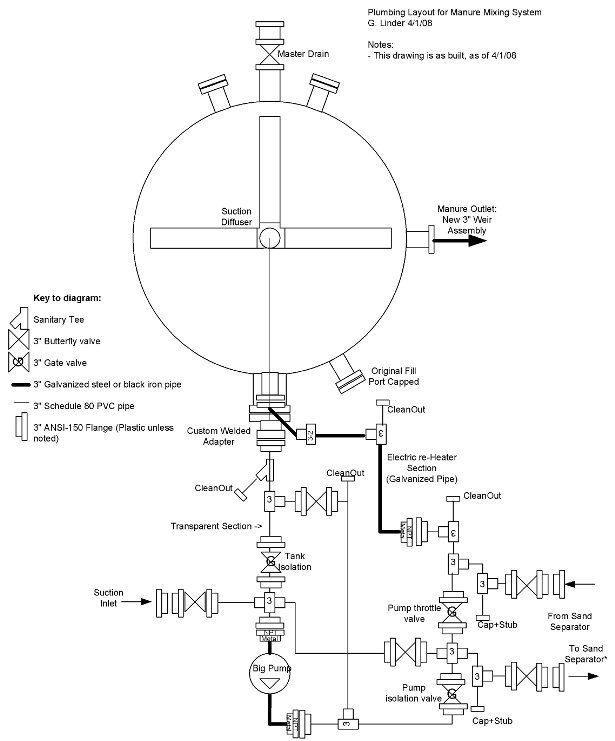
This section contains electrical diagrams for the Clarkson anaerobic digester Version 2. Refer to Section 11.6 for more details on control points and labels.
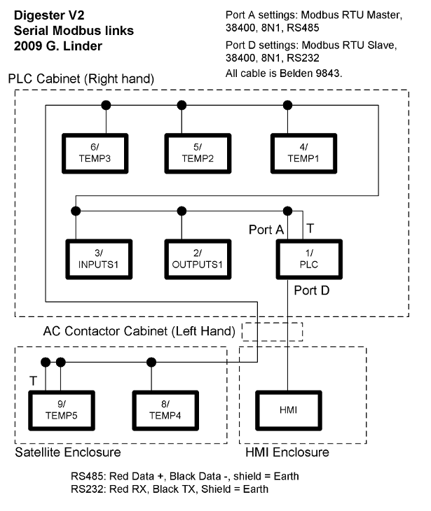
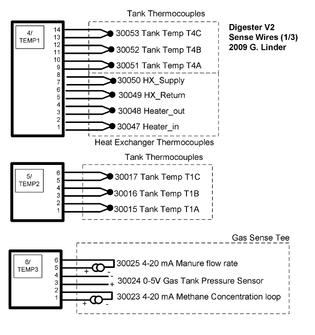
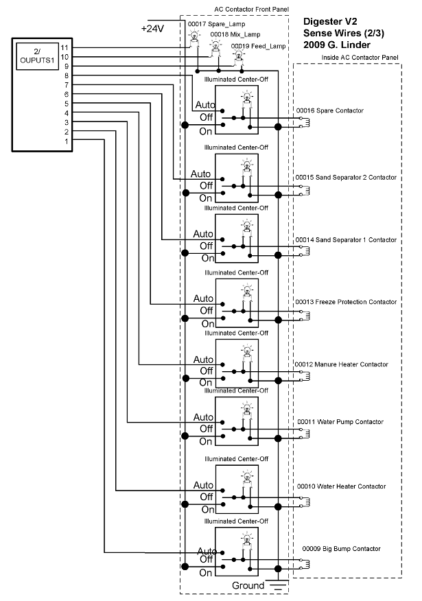
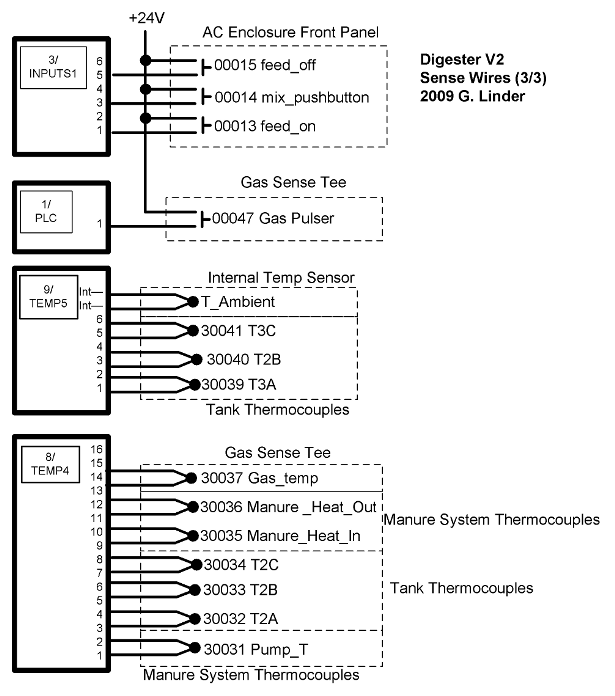
What follows is the specifications of the Version 2 Clarkson Anaerobic digester.
| Manure System
| |
| Tank Dimensions | 4’ diameter, 6’-9” inside height. Total volume, 634 gallons.. |
| Tank Capacity | 515 gallons to “full”, 470 gallons in tank, 45 in plumbing. |
| Feed Rate | 20 Day residence time, 25.75 gallons per day |
| Tank Pressure | 8.3 inches WC(0.3PSI). Tank tested to 27.7 inches WC(1 PSI) |
| Manure Pump | 5 HP Motor @ 240V 3” inlet / outlet chopper pump |
| Manure Flow | 215 GPM max flow. Bypass throttle for control from 0 -> 215 GPM. Pump reverser installed. |
| Pipe Size | All plumbing 3” schedule 80, or schedule 40 PVC or galvanized steel |
| Valves | 3” Wafer-style butterfly or gate-style ductile iron sewerage rated epoxy coated |
| Plumbing Interface | qty. (3) 3” ANSI 150 bolt flanges on various points of system |
| Manure Flow Meter | Dynasonics ultrasonic flow meter on 4 foot galvanized pipe section |
| Mixing | Fully automatic mixing configured by “Mix for SSS seconds ever MM minutes” in PLC |
| Heater System
| |
| Element | 4 kw @ 240V or 3 kw @ 208V |
| Pump | Taco circulating pump: 15 gpm @ 6 PSI rise |
| Pressure | 3 PSI cold, 10 PSI hot, pressured tested to 20 PSI |
| Heater Fluid | Approx. 3 gallons of 50/50 water / propylene glycol mix |
| Temperature | Dual-loop. Tank from ambient -> 50C, Heater fluid, Ambient -> 50 C. Setpoint default 37C |
| Manure Heater | 8 watt per foot self-regulating heater tape, 1400 watts from cold |
| Heater Fluid Flow Meter | 1.25 inch turbine flow meter, 64 pulses per US gallon accessible in PLC enclosure |
| Gas System
| |
| Volume Flow | American Meter AC-250 bellows meter with NP-1 Pulser |
| Methane Concentration | 0-100% optical methane sensor, BCP-CH4 from BlueSens GmbH |
| Heater | Self-regulating heater tape, ~40C design temp. Type T thermocouple installed in sense system |
| Pressure | Adjustable fluid filled back pressure regulator. Default setting 6” WC |
| Electrical System
| |
| Power Requirements | 240 V single phase or 2-phases of 208 V 3-phase. 30 Amps max. Optional 120V outlet |
| Temp Sensors | Type T-Thermocouples in 21 locations |
| PLC | SixNET mIPM w/ 5 instrumentation modules, 16 digital in, 16 digital out |
| Interface | On-board Ethernet for downloading of data. Default IP 10.1.0.1 |
| Data Acquisition | 2 weeks of on-board data storage, all points logged every 10 minutes |
| Control System | Automatic heater and mix control. Semi-automatic feeding system. Automatic load regulation. |
| HMI | Intuitive touch-screen LCD panel for system config parameters |
Copyright © 2007 Mtarri / Varani, used by permission.
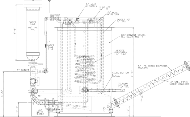
What follows is a table containing the local control points, tag names, and devices addresses utilized in the Clarkson Anaerobic Digester. The Station ID column is presented as “device address / name”. Local Pins describe which physical pins (as labeled on the modules) are connected. Type is what kind of input it is. MODBUS shows the MODBUS address of that device. SixNET shows the SixNET address of that device. Tag Name is the name used in the control firmware to refer to that device, and description describes the device. A MODBUS address starting in “0” is a digital in or out, “3” Is analog in, “4” is analog out.
| Station ID | Local Pins | Type | MODBUS | SixNET | Tag Name | Description |
| 1/PLC | DI1 | 24V DC | 00047 | X46 | Gas_Pulse | Input from pulser |
| Int. | Analog | 30007 | AX6 | meth_volume | Counter for gas pulse | |
| 2/OUTPUTS1 | DO1 | 24V DC | 00009 | Y8 | Big_Pump | Manure pump contactor |
| DO2 | 24V DC | 00010 | Y9 | WaterHeater | Water heater contactor | |
| DO3 | 24V DC | 00011 | Y10 | WaterPump | Water pump contactor | |
| DO4 | 24V DC | 00012 | Y11 | ManureHeater | Manure heater contactor | |
| DO5 | 24V DC | 00013 | Y12 | FreezeProt | Freeze protection contactor | |
| DO6 | 24V DC | 00014 | Y13 | SS1 | Sand Separator 1 contactor | |
| DO7 | 24V DC | 00015 | Y14 | SS2 | Sand separator 2 contactor | |
| DO8 | 24V DC | 00016 | Y15 | Spare | Spare contactor | |
| DO9 | 24V DC | 00017 | Y16 | Spare_Lamp | Spare bushbutton lamp (FEED_OFF) | |
| DO10 | 24V DC | 00018 | Y17 | Mix_Lamp | Mix pushbutton lamp | |
| DO11 | 24V DC | 00019 | Y18 | Feed_Lamp | Feed pushbutton lamp (FEED_ON) | |
| 3/INPUTS1 | DI1 | 24V DC | 00013 | X12 | spare_button | spare pushbutton (FEED OFF) |
| DI2 | 24V DC | 00014 | X13 | mix_button | mix pushbutton | |
| DI3 | 24V DC | 00015 | X14 | feed_button | feed pushbutton (FEED_ON) | |
| 4/TEMP1 | 1-2 | Type T | 30047 | AX46 | Heater_In | Heater inlet temperature |
| 3-4 | Type T | 30048 | AX47 | Heater_out | Heater outlet temperature | |
| 5-6 | Type T | 30049 | AX48 | HX_Return | HX Return temperature | |
| 7-8 | Type T | 30050 | AX49 | HX_Supply | HX Supply temperature | |
| 9-10 | Type T | 30051 | AX50 | T4A | Tank Temp T4A | |
| 11-12 | Type T | 30052 | AX51 | T4B | Tank Temp T4B | |
| 13-14 | Type T | 30053 | AX52 | T4C | Tank Temp T4C | |
| 5/TEMP2 | 1-2 | Type T | 30015 | AX14 | T1A | Tank Temp T1A |
| 3-4 | Type T | 30016 | AX15 | T1B | Tank Temp T1B | |
| 5-6 | Type T | 30017 | AX16 | T1C | Tankl Temp T1C | |
| 6/TEMP3 | 1-2 | 4-20 mA | 30023 | AX22 | meth_conc | Meth Conctration, 0-100% |
| 3-4 | 0-5V | 30024 | AX23 | tank_pressure | Tank Pressure, 0-1 PSI | |
| 5-6 | 4-20 mA | 30025 | AX24 | poop_flow_rate | Poop flow rate, 0-200 GPM | |
| 8/TEMP4 | 1-2 | Type T | 30031 | AX30 | pump_t | Pump Temperature |
| 3-4 | Type T | 30032 | AX31 | T2A | Tank Temp T2A | |
| 5-6 | Type T | 30033 | AX32 | T2B | Tank Temp T2B | |
| 7-8 | Type T | 30034 | AX33 | T2C | Tank Temp T2C | |
| 9-10 | Type T | 30035 | AX34 | Manure_Heat_in | Manure heater inlet temp | |
| 11-12 | Type T | 30036 | AX35 | Manure_Heat_out | Manure heater outlet temp | |
| 13-14 | Type T | 30037 | AX36 | Gas_temp | Gas system temperature | |
| 9/TEMP5 | 1-2 | Type T | 30039 | AX38 | T3A | Tank Temp T3A |
| 3-4 | Type T | 30040 | AX39 | T3B | Tank Temp T3B | |
| 5-6 | Type T | 30041 | AX40 | T3C | Tank Tampe T3C | |
| Int | Internal | 30046 | AX45 | T_Ambient | Ambient Temperature | |
| HMI | Virtual | Boolean | 00025 | Y24 | Mix_enable | Enable / disable auto-mix |
| Virtual | Boolean | 00026 | Y25 | manure_heat_on | Turn on / off manure heater | |
| Virtual | UINT 16 | 4001 | AY0 | T_water_SP | Water temp setpoint | |
| Virtual | UINT 16 | 4002 | AY1 | T_tank_SP | Manure temp setpoint | |
| Virtual | UINT 16 | 4003 | AY2 | mix_time | mix time (secs) | |
| Virtual | UINT 16 | 4004 | AY3 | mix_interval | mix interval (minutes) | |
This section contains the full IEC 61131-3 Functional Block Diagrams requried to implement local control on the Clarkson Version 2 digester. Please refer to Chapter 3 for more details on the application of this information.
Accepts as an input mix_interval and mix_time from the operator interface and outputs mix_interval_T and mix_time_T for use by the timers in MIXCON.
|
|
Accepts as inputs the average tank temperature and water heater input and output numbers from CALCTEMP. HEATCON implements the dual-loop tank heater loop discussed in Chapter 3 Fig. 3.2. Outputs drive the contactors which operate the water pump and water heater.
|
|
Accepts as inputs all six tank thermocouples T1(A,B,C) and T2(A,B,C) and divides the output to form the average tank temperature used in HEATCON. Additionally, averages the two heater output thermocouples, Heater_Out and HX_Supply to form the input data for HEATCON. Accepts T_tank_SP and T_water_SP as inputs from the HMI and ouputs appropriately scaled values for HEATCON.
|
|
This is the functional block diagram which implements both the auto and semi-auto mixing operations, including the manual override and flashing pushbutton indications of activity. Inputs to this routine come from CALCMIX for the timer inputs and the front panels buttons for semi-automatic operation. Outputs control the heater system as a whole, as well as the mixing pump and front panel indications.
|
|
There are many vendors which sell and support cellular data solutions. Among the best looking and apparently most receptive to use with anaerobic digesters include the following:
The website features a suite of web applications called PowerVista, which implements basic SCADA and control room functionality. In addition, they supply the DNP-RTM, a cellular remote terminal unit which would interface directly to the digester’s PLC after a firmware upgrade. Besides this, they are very nice over the phone.
Website: http://www.telemetric.net/ . Postal address: Telemetric, Inc. 9941 West Emerald, Boise, ID 83704. Phone (208)658-1292.
The SensorCast solution is similar to what Telemetric offers, although in a bit of an earlier state of development that Telemetric. The data display and export capabilities SensorCast are better in some ways than Telemetric. They also offer hardware which could interface directly the the Clarkson digester controller with firmware upgrades.
Website: http://www.sensorcast.com/ . Postal address: SensorCast, Inc. 8002 Reeder Rd. Lenexa, KS 66214. Phone (913)492-3726
This vendor offers only cellular data modems. A separate software vendor would be required for data display, although their hardware is among the best and most cost effective in the business.
Website: http://www.bluetreewireless.com/ . Postal address: BlueTree Wireless 30111 Settle Street. Chapel Hill, NC. 27517. Phone (919)928-8033
[1] van Helmont, Jan Baptist. Ortus medicinae, Id est, initia physicae inavidita. Progressus medicinae novus, in morborum, ultionem, ad vitam longam . Amsterdam: Elzever, 1648. Translated by John Chandler, London, England, 1662 in Physick Refined, the common Errors therein Refuted
[2] Mwakaje, Agnes Godfrey. Dairy farming and biogas use in Rungwe district, South-west Tanzania: A study of opportunities and constraints . Renewable and Sustainable Energy Reviews Volume 12, Issue 8, Page 2240.
[3] Environmental Protection Agency, Regulatory Definitions of Large CAFOs, Medium Cafo, and Small Cafos. Available at http://www.epa.gov/npdes/pubs/sector_table.pdf
[4] Market Opportunities for Biogas Recovery Systems: A Guide to Identifying Candidates for On-Farm and Centralized Systems, pp 1. Available at http://www.epa.gov/agstar EPA-430-8-06-004
[5] Power-Technology.com. Comanche 3 Power Station Expansion, CO, USA. [Online]. http://www.power-technology.com/projects/comanche/ . Accessed 04/20/2008.
[6] National Energy Information Administration, Average Wholesale Price by NERC region, 2001-2006. Available at http://www.eia.doe.gov/cneaf/electricity/wholesale/wholesale.html.
[7] National Energy Information Administration, Electric Power Annual 2007: Overview, pp 8. Accessed Feb, 2009. Available at http://www.eia.doe.gov/cneaf/electricity/epa/epa.pdf.
[8] Lusk, P. Methane Recovery from Animal Manures: The Current Opportunities Casebook, pp. 1-2. Resource Development Associates, Washington, DC for NREL.
[9] Gremelspacher, M. Gillespie, G. Welsh, R. North Country New York Dairy Farmer Views on Alternative Energy Production. [Online]. pp. 4. Available: http://web2.clarkson.edu/cbg/docs/Dairy_AD_Summary_Report.pdf. Accessed 09/04/2008
[10] Sheland Farms, Personal Interview with Doug Shelmidine, November, 2008.
[11] Lusk, P. Methane Recovery from Animal Manures: The Current Opportunities Casebook, pp. 4-71. Resource Development Associates, Washington, DC for NREL.
[12] Environmental Protection Agency (EPA) NPDES PERMIT WRITER’S GUIDANCE MANUAL AND EXAMPLE NPDES PERMIT FOR CONCENTRATED ANIMAL FEEDING OPERATION. December 31, 2003. EPA-833-B-04-001.
[13] Federal Register. Part II: Environmental Protection Agency. 40 CFR Parts 9, 122, and 412 Revised National Pollutant Discharge Elimination System Permit Regulation and Effluent Limitations Guidelines for Concentrated Animal Feeding Operations in Response to the Waterkeeper Decision; Final Rule. Vol. 73, No 225. Thursday, Nov. 20, 2008. pp. 70,420
[14] NRCS NRCS National Planning Procedures Handbook. Subpart 600.E.54.A
[15] Harner, J.P. J. Smith. Assessment of Successful Sand-Laden Manure Handling Systems. Sand Systems Conference. East Lansing, Michigan, McLanahan Corporation. November 15-17, 2006.
[16] Nelson, Carl. Lamb, John. Final Report: Haubenschild Farms Anaerobic Digester Updated! August, 2002. The Minnesota Project, Minnesota, MN. http://www.mnproject.org/
[17] Page, David. Modeling Anaerobic Digestion of Dairy Manure. Thesis, 2007. p.54
[18] U.S. Department of Agriculture, Natural Resources Conservation Service. NRCS Conservation Practice Standard 590, April 1999. Nutrient Management.
[19] US Department of Agriculture, Economic Research Service. Manure Management for Water Quality: Costs to Animal Feeding Operations of Applying Manure Nutrients to Land. Agricultural Economic Report Number 824. June, 2003. p. 38
[20] Hickey, Kevin L. Laboratory Scale Anaerobic Digestion of Sand Laden Dairy Manure. Environmental Science and Engineering Program, Clarkson University. July, 2007. p. 2
[21] Linder, Greg. Personal Experience from living in the United States. 1981-2009.
[22] Pell, Alice N. Manure and Microbes: Public and Animal Health Problem? Journal of Dairy Science, Vol. 80 No. 10 1997.
[23] Foster, George McClelland. Traditional Societies and technological change. Harper & Row, 1973. Second edition. pp. 218
[24] Masemola, Kgathane Lowrain. Personal Interview. February, 2008.
[25] Skill Associates. Elimanure webpage. http://www.burnmanure.com/ management/elimanure.html . Accessed 4/8/2009.
[26] Skill Associates. Manure Management: The Power of Green Energy. Powerpoint Presentation, available online. http://www.burnmanure.com/ management/images/skillassoc.pdf . Accessed 4/8/2009.
[27] Caldwell, Emily. Roast your compost. Ag Nutrient Management, 2008. Available online. http://www.progressivedairy.com/anm /features/2008/0508/0508_caldwell.html
[28] Meisterling, Kyle. A broad assessment of manure to power technology and investigation of a potential wind-biogas synergy. Carnegie Mellon Electricity Industry Center Working Paper CEIC-04-03. http://www.cmu.edu/electricity. p. 5
[29] Higman, Christopher. Maarten van der Burgt. Gasification 2nd Edition. Gulf Professional Publishing, 2008.
[30] Rezaiyan, John. Nicholas P. Cheremisinoff. Gasification Technologies: A Primer for Engineers and Scientists. CRC Press: 2005. pp. 50
[31] Rezaiyan, John. Nicholas P. Cheremisinoff. Gasification Technologies: A Primer for Engineers and Scientists. CRC Press: 2005. pp. 13-16
[32] AES Energy. What is Biomass? Website: http://www.aesenergy.net/biomass-energy.html. Accessed 4/8/09.
[33] Haug, Roger Tim. The Practical Handbook of Compost Engineering. CRC Press, 1993. p. 50
[34] Haug, Roger Tim. The Practical Handbook of Compost Engineering. CRC Press, 1993. p. 1
[35] Haug, Roger Tim. The Practical Handbook of Compost Engineering. CRC Press, 1993. p. 48
[36] Van Horn, H.H. et al. Components of Dairy Manure Management Systems. Journal of Dairy Science. Volume 77, No. 7, 1994
[37] Haug, Roger Tim. The Practical Handbook of Compost Engineering. CRC Press, 1993. p. 10
[38] Amon, Thomas, et al. Biogas production from maize and dairy cattle manure- Influence of biomass composition on the methane yield. Agriculture, Ecosystems, and Environment. Elsevier, 2007 Volume 118. pp. 173-182.
[39] Deublein, Dieter. Angelika Steinhauser. Biogas from Waste and Renewable Resources: An Introduction. Wiley-VCH, 2008. pp. 57-65.
[40] Lusk, P. Methane Recovery from Animal Manures: The Current Opportunities Casebook, pp. 2-22 - 2-26. Resource Development Associates, Washington, DC for NREL
[41] Mattocks, Richard. Kintzer, Barry. Wilkie, Ann. AgSTAR Handbook: A Manual for Developing Biogas Systems at Commercial Farms in the United States. 2008. http://epa.gov/agstar/resources/handbook.html Accessed 09/05/08 pp. 2-1
[42] Market Opportunities for Biogas Recovery Systems: A Guide to Identifying Candidates for On-Farm and Centralized Systems, pp 23. Available at http://www.epa.gov/agstar EPA-430-8-06-004
[43] Electric Power Annual 2007 DOE/EIA-0348 (2007). Energy Information Administration Office of Coal, Nuclear, Electric and Alternate Fuels. pp. 11. Washington, DC. [Online] Available: http://www.eia.doe.gov/cneaf/ electricity/epa/epa_sum.html. Accessed 09/22/2008.
[44] Martin, John H. An Evaluation of a Mesophilic, Modified Plug Flow Anaerobic Digester for Dairy Cattle Manure. EPA AgSTAR Program. EPA Contract No. GS 10F-0036K, 20 July 2005.
[45] Chynoweth, David P., Sambhunath Ghosh and Martha L. Packer. Anaerobic Process Literature Review. Journal (Water Pollution Control Federation), Vol. 51 No. 6, 1979. pp. 1200-1214.
[46] Mattocks, Richard. Kintzer, Barry. Wilkie, Ann. AgSTAR Handbook: A Manual for Developing Biogas Systems at Commercial Farms in the United States. 2008. http://epa.gov/agstar/resources/handbook.html Accessed 09/05/08 pp. 1-6
[47] Lusk, P. Methane Recovery from Animal Manures: The Current Opportunities Casebook, p. 3. Resource Development Associates, Washington, DC for NREL.
[48] Cornell Waste Management Institute. Using Manure Solids as Bedding Literature Review. Ithaca, NY: 2006. Cornell University Department of Crop Sciences. Accessed March 2009, http://cwmi.css.cornell.edu/beddinglitreview.pdf
[49] Mtarri / Varani LLC. Clarkson University Model Containment Vessel Fabrication Details Piping Assembly. Mtarri / Varani, LLC. 1511 Washington Street, Golden, CO. 80401.
[50] Mtarri / Varani LLC. Clarkson University Model Containment Vessel Fabrication Details General Arrangement. Mtarri / Varani, LLC. 1511 Washington Street, Golden, CO. 80401.
[51] Clarkson Biomass Group. Research Progress Meeting, Presented to digester research participants, September. 2008.
[52] Clark, Gordon. Reynders, Deon. Practical Modern SCADA Protocols: DNP3, 60870.5 and Related Systems, New York: Newnes, 2004, p. 45.
[53] Weldetnsae, Yotam Tsegay. Heat and Power Optimization for Farm Waste to Energy Conversion, Department of Electrical and Computer Engineering, Clarkson University, May 2008.
[54] Linder, Greg. Care and Feeding of Your New Portable Digester. Self published, 5/9/2008. Available from http://www.linderlabs.com/glinder/innovations/ digv2intro/digesterinstructions.pdf .
[55] Northcote-Green, James. Robert Wilson. Control and Automation of Electrical Power Distribution Systems. CRC Press, 2007. pp 142-146
[56] Brown, Richard E. Electric Power Distribution Reliability. CRC Press, 2002. pp. 24
[57] Masemola, Kgathane Lowrain. Generators for electrical power from farm waste: a thesis, Department of Electrical and Computer Engineering, Clarkson University, Dec 2007.
[58] McFarland, Wayne. North Harbor Dairy Preliminary Cost Estimate - 600 Cows. Stearns and Wheler, LLC. Personal communication, 2/17/09.
[59] CDH Energy Corp. Sheland Farms : Engine Fueled by Anaerobic Digester Project Profile pp. 1, Accessed Feb, 2009. Available at http://cdhnrgy1.user.openhosting.com/Fact%20Sheets/Sheland% 20Farms%20CHP%20Site%20Fact%20Sheet.pdf
[60] New York Independent System Operator (NYISO), FERC Electric Tariff, Original Volume #2. Effective January 2, 2001. Online, http://www.nyiso.com/public/webdocs/documents/ tariffs/market_services/services_tariff.pdf
[61] CDH Energy Corp. Sheland Farms : Engine Fueled by Anaerobic Digester Project Profile pp. 2, Accessed Feb, 2009. Available at http://cdhnrgy1.user.openhosting.com/Fact%20Sheets/Sheland% 20Farms%20CHP%20Site%20Fact%20Sheet.pdf
[62] Clarke, Gordon. Deon Reynders. Practical Modern SCADA Protocols: DNP3, IEC 60870.5 and Related Systems. Newnes, 2004. pp. 1
[63] Clark, G. L. (Larry). Smart Distribution Grid and the Advanced Integrated Distribution Management System(IDMS). Module 4: Deployment of Smarts in the Field: Case Studies from the Alabama Power Perspective. Alabama Power Company, Birmingham Alabama. Presented at 2009 IEEE PSCE Tutorial, Seattle, Washington. March 17, 2009.
[64] New York State Energy Research And Development Authority Distributed Generation / Combined Heat and Power (NYSERDA DG/CHP) homepage. http://chp.nyserda.org/home/index.cfm . Accessed 3/29/09 .
[65] New York State Energy Research And Development Authority Distributed Generation / Combined Heat and Power (NYSERDA DG/CHP) Integrated Data System Users Guide. Available online: http://chp.nyserda.org/support/helpdocs.cfm . Accessed 3/29/09.
[66] New York State Energy Research And Development Authority Distributed Generation / Combined Heat and Power (NYSERDA DG/CHP) Monitoring and Data Collection Standard for NYSERDA DG/CHP Sites . Available online: http://chp.nyserda.org/support/helpdocs.cfm . Accessed 3/29/09.
[67] New York State Energy Research And Development Authority Distributed Generation / Combined Heat and Power (NYSERDA DG/CHP) Summary of Data Requirements for NYSERDA DG/CHP Sites Available online: http://chp.nyserda.org/support/helpdocs.cfm . Accessed 3/29/09.
[68] Linder, Greg. The Importance of Standard SCADA Protocols to the Reliable Operation of Distributed Farm-Scale Anaerobic Digesters. Presented at IEEE PSCE 2009 in Seattle, Washington.
[69] International Telecommunications Union. X.200: Information technology - Open Systems Interconnection - Basic Reference Model: The basic model. Approved 1994-07. Available via download, http://www.itu.int/rec/T-REC-X.200-199407-I/en.
[70] Clark, Gordon. Reynders, Deon. Practical Modern SCADA Protocols: DNP3, 60870.5 and Related Systems, New York: Newnes, 2004, pp. 13-45.
[71] Clark, Gordon. Reynders, Deon. Practical Modern SCADA Protocols: DNP3, 60870.5 and Related Systems, New York: Newnes, 2004, p. 65.
[72] Personal interview, IEEE PSCE 2009 in Seattle, Washington.
[73] New York Independent System Operator. Manual 24: System Analysis Data Manual. Copyright September, 1999. pp. 17
[74] McDonald, John D. Editor. Electric Power Substations Engineering Second Edition. Copyright 2007, CRC Press. pp 7-14 .. 7-15.
[75] Personal interview, Email correspondence with Telemetric, Inc. 03/27/09. http://www.telemetric.net/
[76] Telemetric, Inc. GPRS Data Estimator Rev 1 090326. Provided via email. Contact Telemetric, Inc. http://www.telemetric.net/ . 03/27/09.
[77] Telemetric, Inc. Online demonstration of Telemetric PowerVista software. http://www.telemetric.net/ . Accessed 03/27/09.
[78] Zurawaski, Richard, Editor. The Industrial Information Technology Handbook. Chapter 100. Hu, Zaijun. Eckhard Kruse. Web Services for Integrated Automation Systems – Challenges, Solutions and Future. Copyright 2005.
[79] Dixit, Sudhir. Ramjee Prased. Editors. Wireless IP and Building the Mobile Internet. Artech House Publishers, December 2002. p. 23.
[80] Linder, Greg. AT&T iPhone monthly billing statement, November, 2008.
[81] Telemetric, Inc. Phone conversation with Larry Morrissey. Contact Telemetric, Inc. http://www.telemetric.net/ . 03/14/09.
[82] McDonald, John D. Editor. Electric Power Substations Engineering Second Edition. Copyright 2007, CRC Press. pp 7-2
[83] SixNET, Inc. SIXNET I/O Toolkit. Software documentation. Available in the SixNET SXTools software package, http://www.sixnetio.com/
[84] Eltro Industries/GaugeTech. Shark200 Upgradable Fully Featured Power & Energy Meter. Revenue Grade with Advanced I/O and Power Quality. Marketing Brochure, 2009. Available online: http://www.powermeterstore.com/ crm_uploads/shark200_broshure.pdf
[85] Eltro Industries/GaugeTech. Communicator EXT demonstration software. Free software demo, 2009. Available online: http://www.electroind.com/ em-communicator.html
[86] Hamid, A. Toliyat. G. B. Kliman. Handbook of Electric Motors. 2nd edition, CRC Press, 2004. P. 462